3. Math-FP-Lang Combo#
Objectives: To prepare secondary & tertiary math for my kids
Bad ideas:
distinguish math btw high-school(secondary education) and uni(tertiary education)
distinguish math and science(especially physics)
distinguish math and CS(computer science)
distinguish math and natural language
Good ideas:
Combo of 2nd and 3rd-level math topics
Combo of math and physics
Combo of ‘conventional’ and computational math
Combo of natural language, math language and coding language
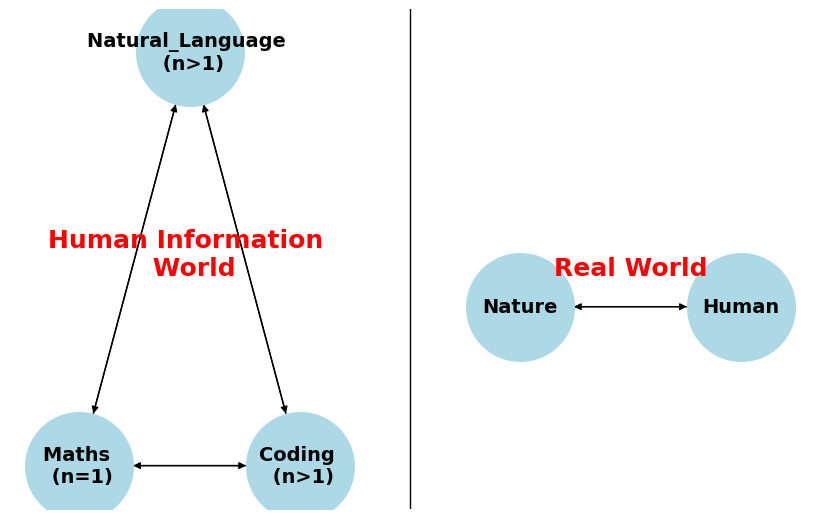
We will follow a worldview as below:
# Draw Two-Worlds
import networkx as nx
import matplotlib.pyplot as plt

G = nx.DiGraph()
edges_left = [("Coding \n (n>1)", "Maths \n (n=1)"), ("Maths \n (n=1)", "Natural_Language \n (n>1)"), ("Natural_Language \n (n>1)", "Coding \n (n>1)"),
            ("Maths \n (n=1)", "Coding \n (n>1)"), ("Natural_Language \n (n>1)","Maths \n (n=1)"), ("Coding \n (n>1)", "Natural_Language \n (n>1)")]
edges_right = [("Nature","Human"),("Human","Nature")]
G.add_edges_from(edges_left)
G.add_edges_from(edges_right)

# Define node positions manually
pos = {"Coding \n (n>1)": (-1, -0.6), "Maths \n (n=1)": (-3, -0.6), "Natural_Language \n (n>1)": (-2, 0.7),
        "Nature": (1, -0.1), "Human": (3, -0.1), }
pos["Human Information \n World"] = (-2, 2)
pos["Real World"] = (3, 2)

plt.figure(figsize=(8, 5))  # Draw the graph
nx.draw(G, pos, with_labels=True, node_size=6000, node_color="lightblue", edge_color="black", font_size=14, font_weight="bold")
plt.text(-2, 0, "Human Information \n World", fontsize=18, ha="center", color='red', fontweight="bold") # Add titles
plt.text( 2, 0, "Real World",              fontsize=18, ha="center", color='red', fontweight="bold")
plt.axvline(x=0, color="black", linestyle="-", linewidth=1) # Draw a vertical line
plt.show()
3.1. Math Foundation - ZFC#
ZFC (see wiki) is the most common math framework, what all we have learned so far are from ZFC:
Zermelo–Fraenkel set theory and the axiom of Choice
In ZFC, three transitions are mathematically sound:
\(\sum\) discrete -> continuous \(\int\): discrete can approximate the continuous (e.g., difference equations to differential equations)
\(\Delta x\) finite -> infinite \(d x\): finite extends to the infinite via limits
series -> formulus: series often condense into formulas where convergent with closed-form formulas
Tools like epsilon-delta proofs, measure theory, and functional analysis ensure rigor across these shifts.
# Discrete to Continuous: Sum vs. Integral
var('x , n')
discrete_sum = sum(1/n^2, n, 1, 10)                    # Finite, discrete
continuous_integral = integral(1/x^2, x, 1, infinity)  # Infinite, continuous
s("Discrete sum (n=1-10):", discrete_sum.n())      # Approx 1.549
s("Continuous integral:", continuous_integral)     # 1

# Finite to Infinite: Partial series vs. full series
finite_series = sum(1/n^2, n, 1, 10)  # Finite
infinite_series = zeta(2)             # Infinite sum = pi^2/6
s("Finite series:", finite_series.n())
s("Infinite series:", infinite_series.n())

# Series to Formula: Taylor series for e^x
series_exp = exp(x).series(x, 5)  # Series
formula_exp = exp(x)              # Formula
s("Series:", series_exp)
s("Formula:", formula_exp)
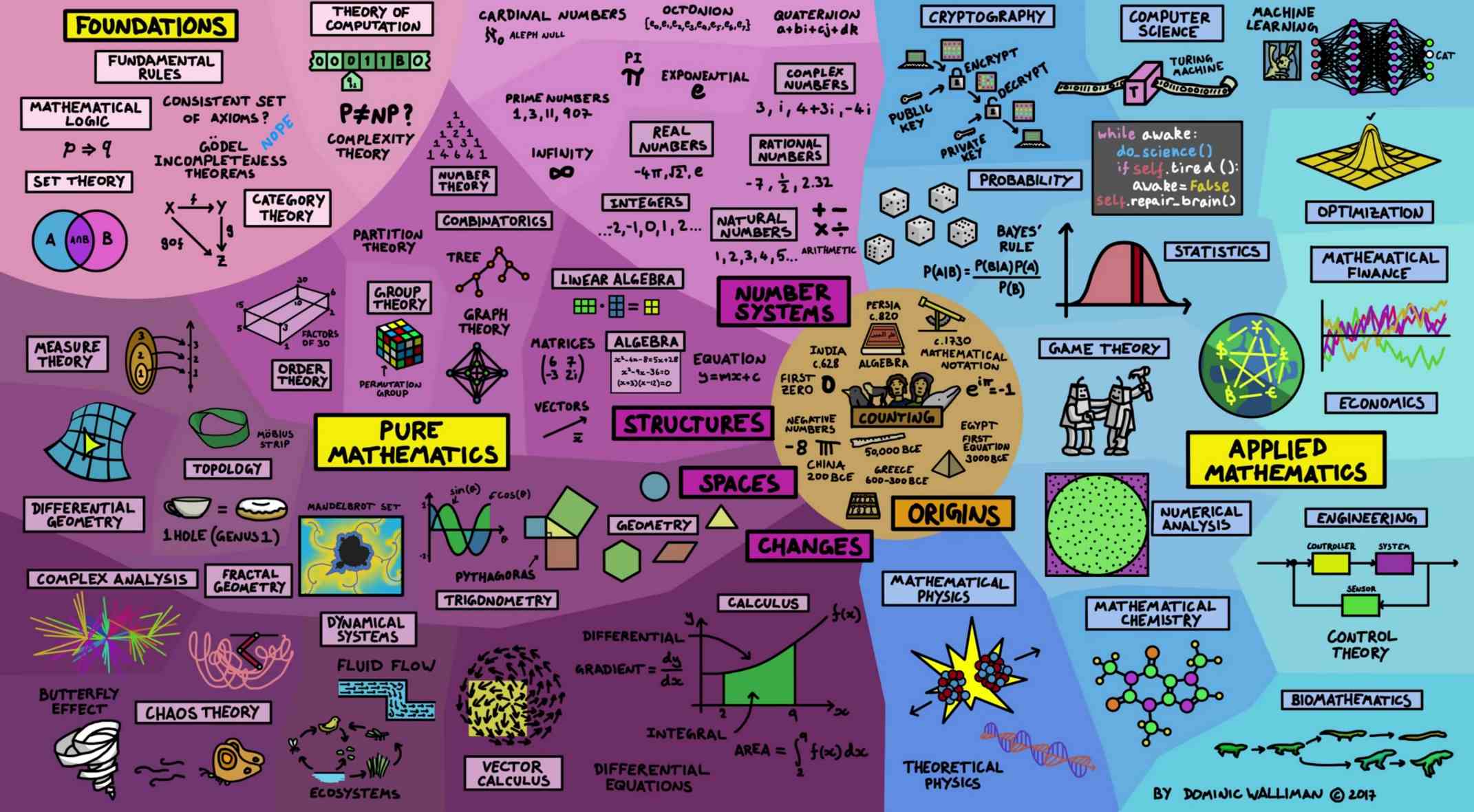
3.2. Mind Map of Math#
Number Theory(Arithmetic)
Algebra
Linear Algebra
Abstract Algebra(Group, Ring, Field)
Combinatorics
Difference(Recursion) & Generating Function
Graph & Network & Algorithm
Calculus & Analysis (Mechanics)
Differential Equations
Topology(First combo of Algebra, Geometry, Analysis)
Functional Programming
Coding Theory & Information
Data analysis
Statistics & Probability Theory
Game Theory & Decision & Operation
Quantum Theory
Symbolic Computation for Sage: covers algebra, computation, and all
how to build a pathway from post-Year 10 math to a freshman mathematician? Y10以后,新州的数学分为四条线,这是非常科学的。但是即使如此,其最难的线(3U4U)还是不足以准备大学预备数学。从初等数学到高等级的数学思维(现代数学)切换有几点需要注意:
离散数学的重要性
离散数学包含的数理逻辑(证明语言),集合论,数论,组合数学,图论等对于理解现代数学的工具多样性非常重要
通过离散数学来掌握高等级数学语言
数学应用或modelling很重要
一定要学习物理或真实世界,所以力学和Simulation/modelling of natural processes非常重要
Python和编程的引入非常重要,Python可以进一步融合物理、数学和真实世界
数学分析(‘连续数学’)虽然重要,但还没必要看数学分析的教材
数学分析的内容主要是定理的证明,不要把自己陷在繁复的计算(微积分)和冗长的证明中
连续数学中,还是要学线代,线性代数不是离散数学,线代 is a form of continuous,但matrix theory在离散数学里面
Human-Info World(triangle:natural language - math language - coding language) VS. Real world
要理解的不止是数学,而是数学描述的真实世界
数学可以讲物理的故事,生物的故事,化学的故事,经济的故事
数学更像一个乐高积木,用数学去微分/积分这个世界
3.3. Online courses#
Coursera平台JHU副教授Joseph Cutrone的课程应用性强, level适合悉悉
Keith Devlin高中水平的数学分析课程 <Introduction to Mathematical Thinking>, mathematical thinking is a powerful cognitive process. School math typically focuses on learning procedures to solve highly stereotyped problems. Mathematical thinking is a way to solve real problems, problems that can arise from the everyday world and science
Prerequisite: High school mathematics. Specific requirements are familiarity with elementary symbolic algebra, number system, some elementary set theory.
MIT LINEAR ALGEBRAThis is a basic subject on matrix theory and linear algebra. Emphasis is given to topics that will be useful in other disciplines, including systems of equations, vector spaces, determinants, eigenvalues, similarity, and positive definite matrices.
Udemy Master Number Theory
Udemy有很多意想不到的课程,相比Coursera,这个平台更自由(除了建制课程,还有很多自由topic,比如lottery math),更个人化(coursera基本是大学老师,课程内容制作僵化不够活泼)
寻找数学应用课程
lottery数学,Google搜:”python lottery analysis”, “number theory behind lottery”
Google/Library genesis搜 ‘scientific computing python’
A Primer on Scientific Programming with Python, Hans Petter, Oslo兼数学、算法numerical methods、python的经典,16年就出到第五版,因作者去世衍生了近年一系列书
本书课件网站包含pdf和ipynb多形式slides
算法numerical methods常包括:Linear Algebra and Systems of Linear Equations, Eigenvalues and Eigenvectors特征值特征向量, Least Squares Regression, Interpolation插补, Taylor Series, Root Finding, Numerical Differentiation/Integration, Ordinary Differential Equations (ODEs) Initial-Value Problems, Boundary-Value Problems for ODEs, Fourier Transform
Onlinebook Mathematical Python包括数论基础的logic, prime numbers, divisors 到 数值积分和ODEs的内容
Onlinebook Calculus with Python – A Tiny Little Book
Google ‘number theory python’
An Illustrated Theory of Numbers 已下pdf书和ipynb笔记,兼有图解数论和python数论
A-level (edx)
Year 13 - Course 1: Functions, Sequences Series, Numerical Methods(全部有python实施)
Year 13 - Course 2: General Motion, Moments Equilibrium, Normal Distribution, Vectors, Differentiation, Integration
Further Y12 - C1: Complex Numbers, Matrices, Roots of Polynomial Equations and Vectors
Further Y12 - C2: Matrices, Induction, Calculus Applications, Maclaurin Series, Complex Numbers, Polar Coordinates
Further Y13 - C1: ODE, Further Integration, Curve Sketching, Complex Numbers, Vector Product Further Matrices
Further Y13 - C2: ODE, Momentum, Work, Energy & Power, Poisson, Central Limit Theorem, Chi 2 Tests, Type I II Errors
最佳物理融合所有数学Mathematical and Computational Methods
Calculus review The Greeks and the development of the limit The logarithm and the revolution of numerical computation from tables The concept of the derivative and antiderivative How to integrate Multivariable integrals Frullani and Gaussian integrals Feynman integration
Vector calculus Vector fields The divergence theorem Stokes theorem Gradient Laplace’s equation
Complex analysis Complex numbers Analytic functions Cauchy’s theorem Calculus of residues
Linear Algebra Matrix multiplication The determinant Matrix inverses Eigenvalues and eigenvectors Abstract vector spaces with inner products
Differential equations First-order linear differential equations First-order nonlinear differential equations Differential equations with constant coefficients Variation of parameters Method of undetermined coefficients Frenet-Serret apparatus
Fourier series Dirichlet theorem and Fourier summation formula Poisson’s theorem
3.4. 名词解释#
离散数学 VS. 连续数学(微积分和分析)
离散数学是数学几个分支的总称,包含数理逻辑(真值表,证明),集合论,信息论,数论(密码学),组合数学,图论,抽象代数,拓扑学,运筹学,博弈论决策论、效用理论、社会选择理论。
在现代,计算机科学的数学就是离散数学,数值分析是离散数学的重要应用。
广义的组合数学(Combinatorics)相当于离散数学,狭义的组合数学是组合计数、图论、代数结构、数理逻辑等的总称。组合数学是一门研究可数或离散对象的科学。
B站找到“乐乐课堂” 很多好视频
分析学和数学分析:
分析学Analysis,把数学当做一门语言来定义,我们最熟悉函数的解析,实数序列和级数的极限论,幂级数和函数论,度量空间或衍生的拓扑向量空间的知识
微积分是分析的衍生学科,也就是分析在几何上的应用部分
狭义理解,分析学就是实分析Real analysis(实数的数学分析),数学分析的基础,从极限到全纯函数
数学分析,则主要是为了把分析和逻辑学,哲学上的分析作区分。即用数学角度建立并使用数学对象,直接分析数学问题并间接分析实际问题,数学分析是20世纪才有的
数学分析假设但你知道有理数(不知道实数),教你如何从有理数构建实数,又证明了极限这个概念在R上是自洽的,于是你可以放心大胆的在R上用极限运算。
微积分是假设你已知道实数,并且告诉你极限运算可以在R上用,于是你就可以calculate啦
微分
运动是visible(本质是空间位移),一阶导是速度,二阶导是加速度
多元微积分 or 多变量微积分(Multivariable calculus,multivariate calculus): 偏微分(partial)和全微分(total)
Wiki上偏导数和偏微分是同一词条
微分在牛顿发明的时候很简单(“微分”曲型面积来求解),150年后又用极限limit概念“重新发明”了微分(以柯西数列做基础的微积分-多矩形对面积的逼近&数列到极限)
-
描述某一类函数与其导数之间的关系。微分方程的解是一个符合方程的函数 y=f(x),初等代数方程里解是常数值
只有少数简单的微分方程可以求得解析解analytical expression,二次方程的根就是一个解析解的典型例子(初等代数方程里解析解也被称为公式解)
用数值分析的方法电脑求近似值(数值解)。大多数偏微分方程,尤其是非线性偏微分方程,都只有数值解。
常微分方程ordinary differential equation只包含一个变量,相对应偏微分方程partial differential equation包含多个变量,求偏导数
和差分方程的理论有密切的关系, 差分方程(difference equation)的坐标是离散值,差分方程研究递推关系(Recurrence relation)
经典: population growth model(马尔萨斯模型), logistic模型, Solow模型, 牛顿第二定律
Category theory 范畴论:以抽象的方法来处理数学概念,将这些概念形式化成一组组的“对象”及“态射”
Set theory 集合论: 数理逻辑I只涉及一阶逻辑这个完备体系下的问题,尽管关系是用集合的方式表示,但是并不依赖集合论的知识。而数理逻辑II的才会讨论更一般的问题,其第一,也是最主要的部分就是集合论。所以可以把学习路线简化为: 数理逻辑的完备部分 -> 集合论 -> 数理逻辑的不完备部分
集合, 就是把一堆东西放在一起, 之间的互相作用我们称之为操作或者运算
群 = 集合 + 运算
Group theory 群论:刻画结构的一种非常基础的工具。应用: 魔方,正交表,高次方程解析解,密码学,拓扑基本群
Measure theory 测度论:测度论是实分析的基础,就好比实数理论之于数学分析。传统的积分是在区间上进行的,后来人们希望把积分推广到任意集合上,就发展出测度的概念。
实变函数的核心是勒贝格积分,而勒贝格积分是黎曼积分的推广。黎曼积分的核心思想是分割积分区间然后求黎曼和取极限,如极限存在则称函数为黎曼可积的。但是黎曼积分有很大的局限性,他对函数的性态要求很高,要求函数几乎处处连续。
勒贝格积分的思想跟黎曼积分不同,他不分割函数的积分区间,而是分割函数的值域区间,然后乘以对应积分区间的测度求和取极限。测度论是用来度量积分区间的,输入一个积分区间,测度函数给出一个正的实数。对于一维空间来说,测度就是区间的长度,对于二维区间来说,测度表示积分区域的面积,对于三维空间,测度表示积分区间的体积,对更高维的空间来说,测度代表类似体积的东西。可见测度论是实变函数的核心理论。
测度论是概率论的理论基础
Order theory 序理论
Graph theory 图论:
Complex analysis 复分析:the branch of mathematical analysis that investigates functions of complex numbers 复变函数
实分析中的泰勒级数和傅里叶级数, 这两者都是关于某个函数的级数展开式, 两者的系数分别是通过求导和积分得出来的, 实数世界里两者毫不相关, 复分析却告诉我们:它们是同一个东西!只是将其在不同的角度“投影”到实数世界里,就产生了不同的“物像”。所以复数揭示了微分与积分的一种隐藏的联系–即全纯函数微分与积分等价
Functional analysis 泛函分析:
Vector calculus 向量分析,或向量微积分,“向量分析”有时也用作多元微积分的代名词,包括向量分析,偏微分和多重积分等多元实分析