13. Math Computational Methods#
MCM is a Mathematical Physics course used as the math foundation of Quantum Mechanics.
Physics is naturally speaking math.
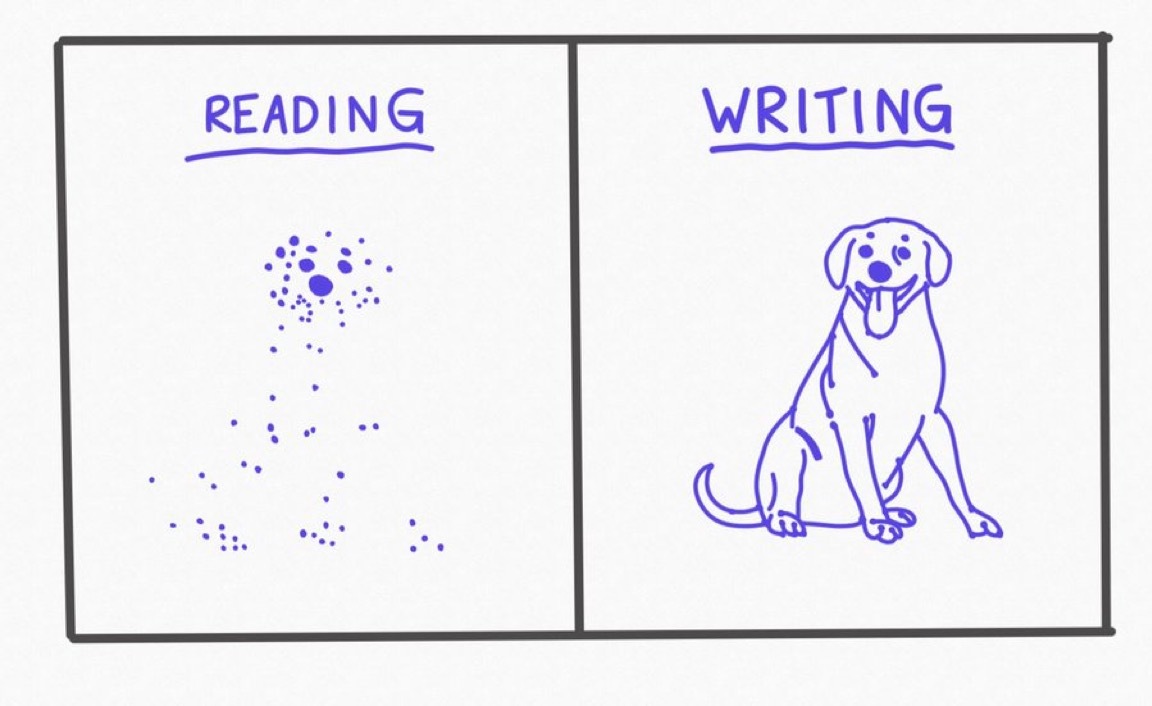
Power of output
13.1. Calculus#
13.1.1. Review#
The essential of Calculus is how God building this world
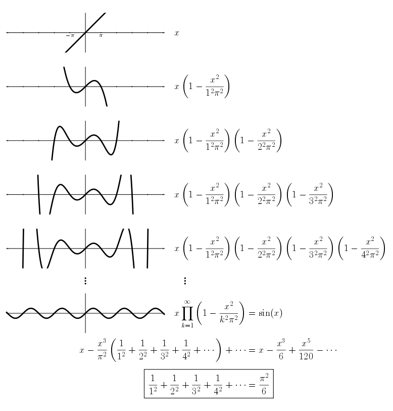
Euler Solution to Basel Problem Euler used infinite products that is similar to Taylor expansion

The difference between Taylor series and MacLaurin series:
Taylor series can be expanded at any \(x\) and are more generalized
Maclaurin series are always expanded at \(x= 0\)
Ten Important Identities
The quadratic equation : \(ax^2+bx+c\) has 2 roots \(r=\large\frac{-b\pm\sqrt{b^2-4ac}}{2a}\)
Fundamental trigonometric identity : \(\cos^2{\theta}+\sin^2{\theta}=1\)
Trigonometric Definitions : \(\sec{\theta}=\frac{1}{\cos{\theta}}\quad\tan{\theta}=\frac{\sin{\theta}}{\cos{\theta}}\quad\csc{\theta}=\frac{1}{\sin{\theta}}\quad\cot{\theta}=\frac{\cos{\theta}}{\sin{\theta}}\)
Double Angle Formulae : \(\cos{2\theta}=\cos^2{\theta}-\sin^2{\theta}\quad\sin{2\theta}=2\sin{\theta} \cos{\theta}\)
Factorization of the difference of squares : \(x^2-a^2=(x+a)(x-a)\)
Geometric Series : \(\large\sum^{\infty}_{n=0}x^n=\frac{1}{1-x}\)(very useful) for \(|x|<1\) and \(\Sigma^{N}_{n=0}x^n= \frac{N!}{n!(N-n)!}x^{N-n}y^n\) for all \(x\).
Binomial Theorem : \((x+y)^N=\sum^{N}_{n=0}\begin{pmatrix}N\\n\end{pmatrix}x^{Nn}y^n=\Sigma^{N}_{n=0}\frac{N!}{n!(N-n)!}x^{N-n}y^n\)
see Binomial Pyramid
Power series for the exponential : \(e^x=\Sigma^{\infty}_{n=0}\frac{1}{n!}x^n\)
Relation for trig functions to exponentials : \(\cos{\theta}=\frac{1}{2}(e^{i\theta}+e^{-i\theta})\) and \(\sin{\theta}=\frac{1}{2i}(e^{i\theta}-e^{-i\theta})\)
Relation of hyp functions to exponentials : \(\cosh{x}=\frac{1}{2}(e^x+e^{-x})\) and \(\sinh{x}=\frac{1}{2}(e^x-e^{-x})\)
See coding translation:
# 6 Geometric
var('x,n')
f = x^n
geo = sum(f,n,0,oo, hold=True)  # oo Infinity
s(geo)

# 7 Binomial
sum1 = sum(binomial(n,x),x,0,n, hold=True) # hold=True: before evaluating
s(sum1 == sum1.unhold())

# 8 Power Series of e
epow = sum(x^n/factorial(n),n,0,oo, hold=True)
s(epow == epow.unhold())

# converged limit of pi
ff = sqrt(sum(6/n^2 ,n,1,oo, hold=True))
s(ff == ff.unhold().n())
Formulae
T Formulae
\(\large t=\tan{\frac{x}{2}}\)
\(\large\sin{x}=\frac{2t}{1+t^2}\)
\(\large\cos{x}=\frac{1-t^2}{1+t^2}\)
\(\large\tan{x}=\frac{2t}{1-t^2}\)
\(\large dx=\frac{2}{1+t^2}dt\)
Video notes
The much less known inverse pythagoras theorem is \(\large\frac{1}{a^2}+\frac{1}{b^2}=\frac{1}{h^2}\).
The sum of the series \(\sum_{j=1}^nj=\large\frac{n(n+1)}{2}\)
The sum of the series \(\sum_{j=1}^nj^2=\large\frac{n(n+1)(2n+1)}{6}\)
From the sum of the 2 previous series \(\sum_{j=1}^nj^3=\large\frac{n^2(n+1)^2}{4}\)
For trigonometric substitution, both \(x=\sin{\theta}\) and \(x=\cos{\theta}\) can be used but use second option.
Gaussian Integral : \(\large\int_{-\infty}^{\infty}dx\ e^{-x^2}=\sqrt{\pi}\)
Frullani Integral(useful) : \(\large\int_0^{\infty}\mathrm{d}x\frac{f(ax)-f(bx)}{x}=(f(0)-f(\infty))\ln{\frac{b}{a}}\)
All Pythagorean triplets can be found by using the formula \(z\) -> \(z^2\) where \(z\) is a complex number. The method also requires multiplying by \(\frac{1}{2}\) or integers.
Trigonometric Substitutions
For integrals containing a term \(ax+b\), use \(u=ax+b\)
For integrals containing a term \(\sqrt{a^2-x^2}\), use \(x=a\sin{\theta}\text{ or }x=a\cos{\theta}\)
For integrals containing a term \(\sqrt{a^2+x^2}\), use \(x=a\sinh{u}\text{ or }x=a\tan{\theta}\)
For integrals containing a term \(\sqrt{x^2-a^2}\), use \(x=a\cosh{u}\)
For integrals \(\int\frac{1}{a+b\cos{\theta}}\) or \(\int\frac{1}{a+b\sin{\theta}}\), use t-formula
Substitution : \(t=\tan{\frac{\theta}{2}}\)
\(\sin{\theta}=\frac{2t}{1+t^2}\)
\(\cos{\theta}=\frac{1-t^2}{1+t^2}\)
For integrals \(\large\int\frac{1}{(px+q)\sqrt{ax^2+bx+c}}\), use \(\frac{1}{u}=px+q\)
To find the area bounded by a parametric curve, go to A-level-further-Module-5
Mass for sphere :
\(M=\int_0^Rdr r^2\rho_0\int_{-1}^1d\cos{\theta}\int_0^{2\pi}d\phi\)
where \(\rho_0\) is a constant in \(\rho(r)\).
Feynman Method :
Insert a parameter (e.g. \(\alpha\)) and evaluate if at a constant (e.g. \(\alpha=1\)) then you have to add a \(\large\frac{d^m}{d\alpha^m}\) when you integrate the terms with \(m\).
Formula for the moment of inertia :
- \[I=\int d^3r\rho(\bf r)r^2_ \perp(\bf r)\]
where \(\rho(\bf r)\) the mass density at the position \( \bf r\) and \(r_\perp(\bf r)\) is the perependicular distance of the position vector at \(\bf r\) to the rotation axis for the moment of inertia.
For sphere of d dimensions :
D-dimensional vector is \(x=(x_1,x_2,\ldots,x_{d-1},x_d)\)
Spherical Coordinates : \({r(\text{radius?}),\theta_1,\theta_2,\ldots,\theta_{d-1}}\)
Which satisfies : \(x_1=r\cos{\theta_1}, x_2=r\sin{\theta_1}\cos{theta_2}, x_3=r\sin{\theta_1}\sin{\theta_2}\cos{\theta_3},\ldots,x_{d-1}=r\sin{\theta_1}\sin{\theta}_2\ldots\cos{\theta_{d- 1}}\)
And also \(x_d\) is the same as \(x_{d-1}\) except the \(\cos\) is a \(\sin\)
Volume of d-sphere : \(V_d=\int_0^Rdrr^{d-1}\int_0^\pi d\theta_1\sin^d_2{\theta_1}\) where sequence has \(\theta_n\) increasing to \(\theta_{n+1}\) and \(\sin\) power decreasing each time by 1 down to 1. Last integral in product : \(\int_0^{2\pi}d\theta{d-1}=2\pi\)
Work out integrals of form \(\int_0^pi d\theta\sin^\alpha\theta=I(\alpha)\)
\(\alpha I(\alpha)=(\alpha-1)I(\alpha-2)+2\delta_{\alpha=1}\)
13.1.2. Problem Set 4#
var('n z')
f=(-1)^n*(n+1)*z^(2*n)
sum1=sum(f,n,0,oo,hold=True)
s(sum1==sum1.unhold())
expand((3390-x)^3)
-x^3 + 10170*x^2 - 34476300*x + 38958219000
how to derive? and present math formula
f(x)=2^(x-1)*binomial(10,x)
for i in range(1,11):
    print(f(i))
10
90
480
1680
4032
6720
7680
5760
2560
512
13.1.3. Week 4#
\(I_{cylinder} = 2\pi \rho \int_0^h dz \int_ 0^R dr\, r^3 = \frac{1}{2}\rho \pi R^4h\)
For center of mass, integrate over the density formula times the dimension(e.g. for x-coordinates, multiply by x). Center of mass can then be used for moment of inertia.
n,r,R,M – those are commonly occupied by PC, so use full-word, like “Mass” et.al
# 3D integral
var('r theta phi R rho_0')
M = integral(integral(integral(rho_0*r^2*sin(theta), phi, 0, 2*pi, hold=True),
                                theta, 0, pi, hold=True),
                                r, 0, R, hold=True)
s(M == M.unhold())

r,R,M=var('r,R,M')
#s(n(sqrt(pi)/4))
#s(n(sqrt(3)*3*5*7*9*11/2^6))
s(integral(2*pi*M/(pi*R^2)*r^3, r))
13.1.4. Week 3#
a=4
s(integral(1/(a^2+x^2), x, 0, a))
s(diff(sqrt(1-x^2), x))
s(integral(sec(x)^3, x))
s(n((ln(1+1/sqrt(2))-ln(1-1/sqrt(2))+4/sqrt(2))/4))

f(x)=x*sinh(x)-cosh(x)
a=(e^2+e^(-2))/2
s(n(2*pi*(f(a)-f(1))))
s(n(integral(x*cosh(x), x, 1, cosh(2))*2*pi))
s(n(integral(x*sqrt(1+(1/(3*x^(2/3)))^2), x, 0, 1)*2*pi))
s(n(sqrt(2)*pi))
s(n(integral(x*sqrt(1+4*x^2), x, 0, 1)*2*pi))
s((x^2/(x^4-16)).partial_fraction())
s(integral(4/(x^2+4), x))
s(diff((2*arctan(x/2)-ln(x+2)+ln(x-2))/8, x))
s(simplify(diff(arcsin(x)-x*sqrt(1-x^2), x)))
s(diff(sqrt(e^x), x))
s(diff(2*ln(e^(x)), x))
13.1.5. Week 2#
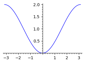
plot(1-cos(x), (x, -pi, pi), figsize=3)
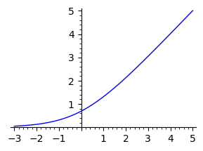
plot(ln(e^x+1), (x, -3, 5), figsize=3)
var('a,n')
f=((-1)^n*x*(a*x)^(2*n+1))/factorial(2*n+2)
sum1=sum(f,n,0,oo,hold=True)
s(sum1 == sum1.unhold())
var('n,a')
f=((-1)^n*(a*x)^(2*n+1))/factorial(2*n+1)
sum1 = sum(f,n,0,oo, hold=True) # hold = before evaluating
s(sum1 == sum1.unhold())
a,n,x = var('a,n,x')
f=((-a)^n*x^(n+1))/factorial(n+1)
sum1 = sum(f,n,0,oo,hold=True)
s(sum1 == sum1.unhold())
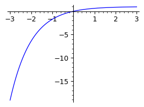
# Every point on the curve can expand to a Taylor series
plot(1-e^-x, (x, -3, 3), figsize=3)
x1=5.99580197536
x2=6.05575999511
x3=3.83164672531
x4=3.86996319256
a=6.02-x1
b=x2-x1
c=a/b
d=180+c
f=d*0.75
g=f-135
h=x4-x3
j=x3+g*h
s(a)
s(b)
s(c)
s(d)
s(f)
s(g)
s(h)
s(j)
def sum_recp(n):
    ans=0
    for i in range(1, n+1):
        ans+=1/i
    return ans
for j in [5, 10, 15, 20]:
    print(n(sum_recp(j)))
13.1.6. Week 1#
g=9.81
v=3.64/sqrt(3/g)
theta=23*pi/180
vx=v*cos(theta)
vy=v*sin(theta)
t1=vy/g
s1=g/2*t1^2
s2=s1+1.5+0.05*sin(theta)
t2=sqrt(2*s2/g)
t=t1+t2
d=vx*t
print(n(d))
s(expand((1+(x^2/2-x^4/24+x^6/720)+(x^2/2-x^4/24+x^6/720)^2+(x^2/2-x^4/24+x^6/720)^3)*(x-x^3/6+x^5/120-x^7/5040)))
s(n(sin(pi/4)))
f(x)=x-x^3/factorial(3)+x^5/factorial(5)-x^7/factorial(7)+x^9/factorial(9)
s(n(f(0)))
s(n(f(pi/4)))
s(n(f(pi/2)))
Projectile problem - Correct solution:
d=pi/180
x,y=var('vy,ty')
s=solve([ vy*ty==(200-4*sin(35*d)), vy==9.8*ty ],vy,ty,solution_dict=True)
vy=s[1][vy]
ty=s[1][ty]
D=vy*(cos(35*d)/sin(35*d))*(ty+sqrt(200*ty/vy))
print(D.n())
566.339564823947
plot(x/sin(x), (x, -pi, pi), figsize=4, ymin=0, ymax=7)
f(x)=1/(1+e^x)
show(plot(f(x), (x, -5, 5), figsize=3))
show(plot(f(x)+f(-x), (x, -5, 5), figsize=3))
show(plot(f(x)-f(-x), (x, -5, 5), figsize=3))
show(plot(diff(f(x)), (x, -5, 5), figsize=3))
show(plot(f(x)*(1-f(x)), (x, -5, 5), figsize=3))
show(plot(f(x)*f(-x), (x, -5, 5), figsize=3))
show(plot(x/sin(x), (x, -5, 5), figsize=3, ymin=-5, ymax=5))
s=7
x=2
for i in range(5):
    x=(x+s/x)/2
    print(n(x))
print(n(sqrt(s)))
13.2. Midterm 1-3#
for checking answers
f=integral(x^4,x,0,1)
g=integral((1-x^2)^2,x,0,1)
h=integral(x^2*(1-x^2),x,0,1)
s(n(h/sqrt(f*g)))
s(desolve((6*x^2*y+4*y^3)*diff(y,x)+4*x^3+6*x*y^2==0,y,show_method=False))
var('t x')
assume(t>0)
s(integral(x^2*e^(x^3),x,0,t))
y=function('y')(x)
s(desolve(diff(y,x)+3*x^2*y==x^2,y,show_method=False))
A=matrix(3,3,[2,4,1,-2,4,3,-3,6,5])
B=matrix(3,3,[2,-14,8,1,13,-8,0,-24,16])/8
s(A.inverse()==B)
A=vector([1,1,1])/sqrt(3)
B=vector([1,-1,0])/sqrt(2)
C=vector([1,1,-2])/sqrt(6)
s(A.cross_product(B)==C)
var('t z')
s(diff((z-x)*e^(i*t*z),z))
var('x y')
s(diff(y/(x^2+y^2),y))
var('a')
s(diff(3^x,x))
s(n((24*ln(2)-7)/9))
plot((x^5-1)/ln(x),(x,0,1),figsize=3)
13.3. Vector Calculus#
13.3.1. Review#
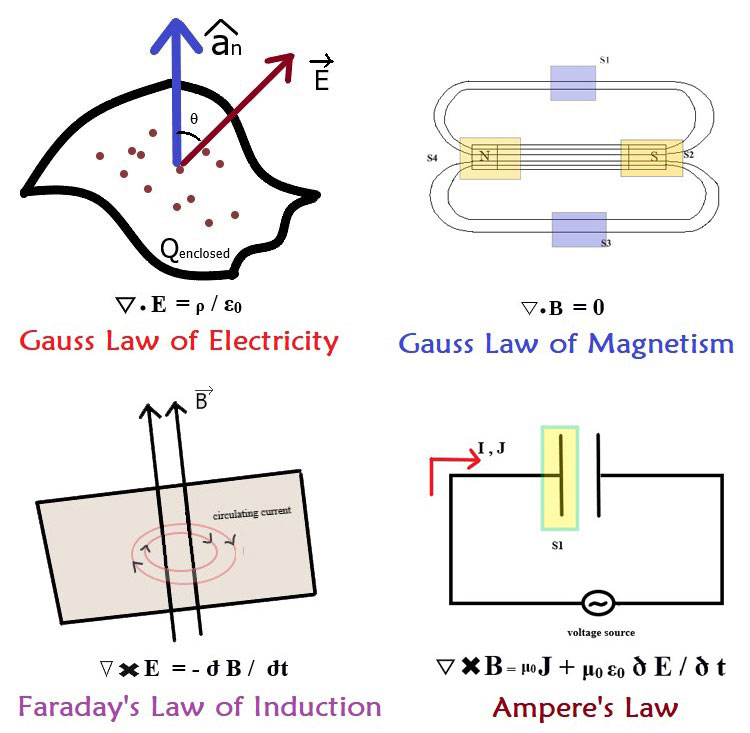
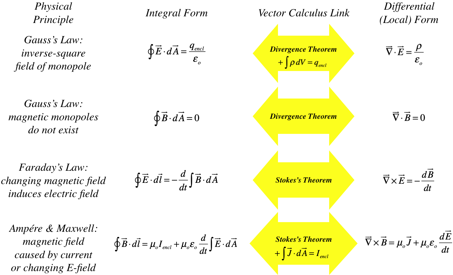
Maxwell eq:
Gauss’s law for static electric fields (\(E\))
Gauss’s law for static magnetic fields (\(B\))
Faraday’s law which says a changing magnetic field (over time) produces an electric field
Ampere-Maxwell’s law says a changing electric field (over time) produces a magnetic field
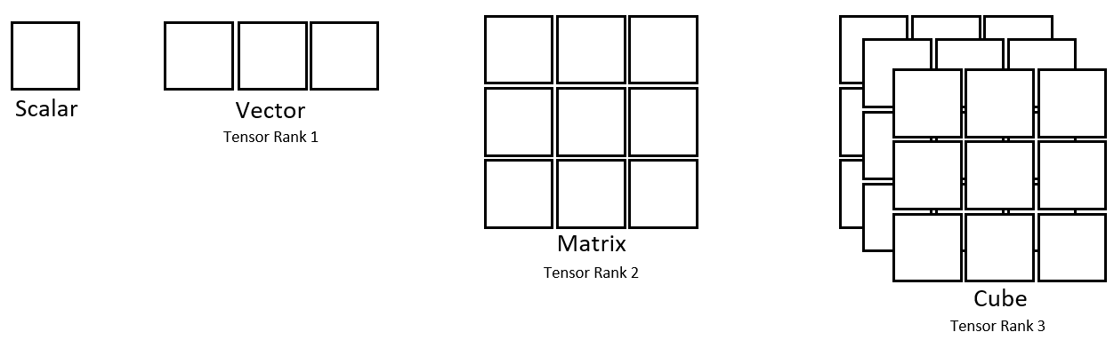
Field Theory
Scalar field -> Vector field -> Tensor field
a scalar field has 1 value at a given point of a mathematical space (e.g. Euclidean space or manifold),
a vector field has 2 (direction and magnitude), vector field is a special case of a tensor field, or a tensor field of rank 1.
a tensor field has 2+ (e.g. represented by an ellipse at each point with semi-major axis length, semi-minor axis length, and direction)

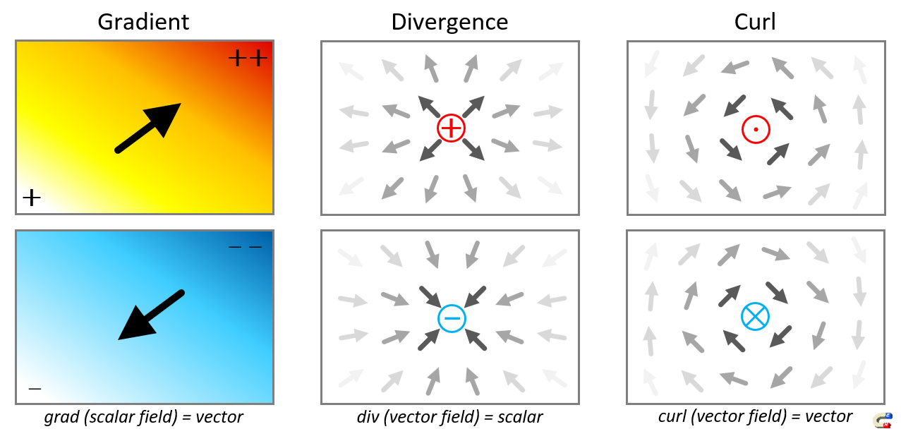
Scalar field has math modelling - Grad
Vector field has two-forms of math modelling (use separately or combined):
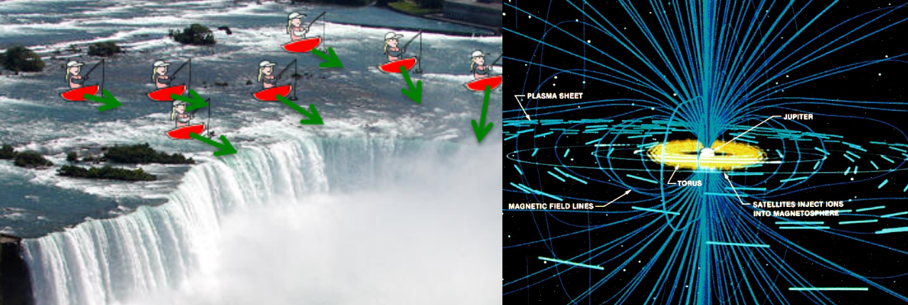
connecting to a point, converge or diverge - divergence (e.g. electric charge);
physical meaning?
rotating a point - curl (e.g. cyclone, solar, galaxy)
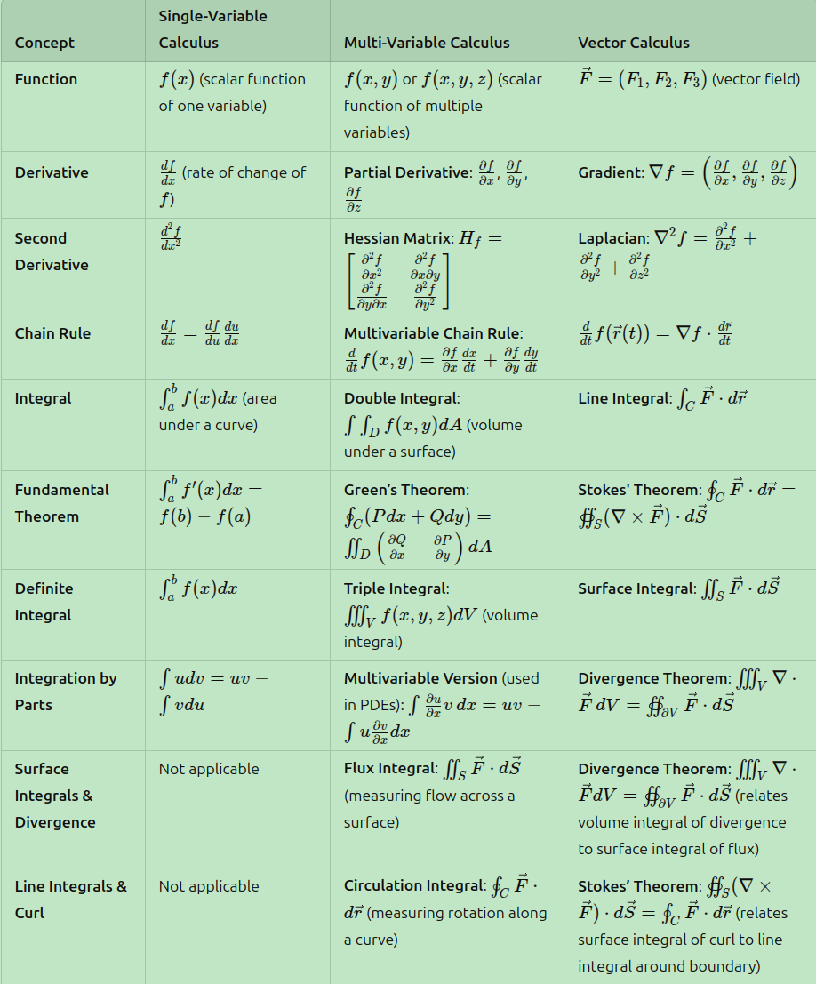
Comparison of single-var, multi-var, vector calculus
vector calculus is usually treated as 3D multi-var calculus
The universe try to tell us that when you integrate the “derivative” of a function within a region
where the type of integration/derivative/region/function involved might be multidimensional, but what you get just depends on the value on boundary function of that region
this is one of the most beautiful things in the universe.
Formula |
Solution |
dimensional reduction |
|---|---|---|
Newton-Leibniz formula |
1D -> dot |
\(\int_a^b f(x)dx=F(b)-F(a) \) |
Green theorem |
2D -> 1D |
\(\iint_D (-\frac{\partial P}{\partial y} + \frac{\partial Q}{\partial x})dxdy = \oint_{\partial D} Pdx + Q dy\) |
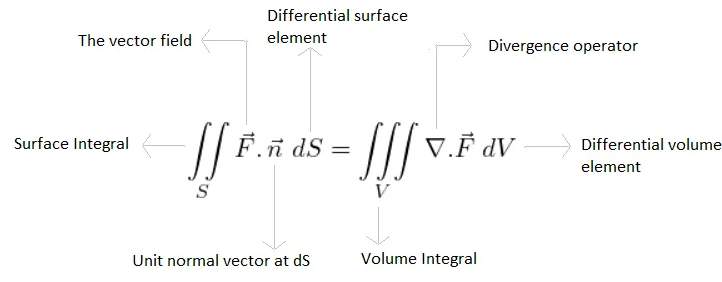
Gauss (Gauss’ flux theorem) |
3D -> 2D |
\(\iiint_D (\frac{\partial P}{\partial x} + \frac{\partial Q}{\partial y} + \frac{\partial R}{\partial z})dxdydz = \oint_{\partial D} Pdydz + Q dzdx + R dxdy\) |
Divergence theorem |
nD -> 3D |
|
Generalized Stokes formula |
manifolds |
\(\int_M d\omega = \int_{\partial M} \omega \) |
Notes
Div & Curl omitted
Line integral : Related to arc length so formula is \(I=\large\int_a^bds\vec{F}\cdot\hat{t}=\int_{x_a}^{x_b}dx\sqrt{1+(\frac{df}{dx})^2}\vec{F}(x)\cdot\hat{t}\)
\(\hat{t}\) is the tangent vector to path.
\(\vec{F}\) is the vector field.
Then use arc length formula or second section for the line integral.
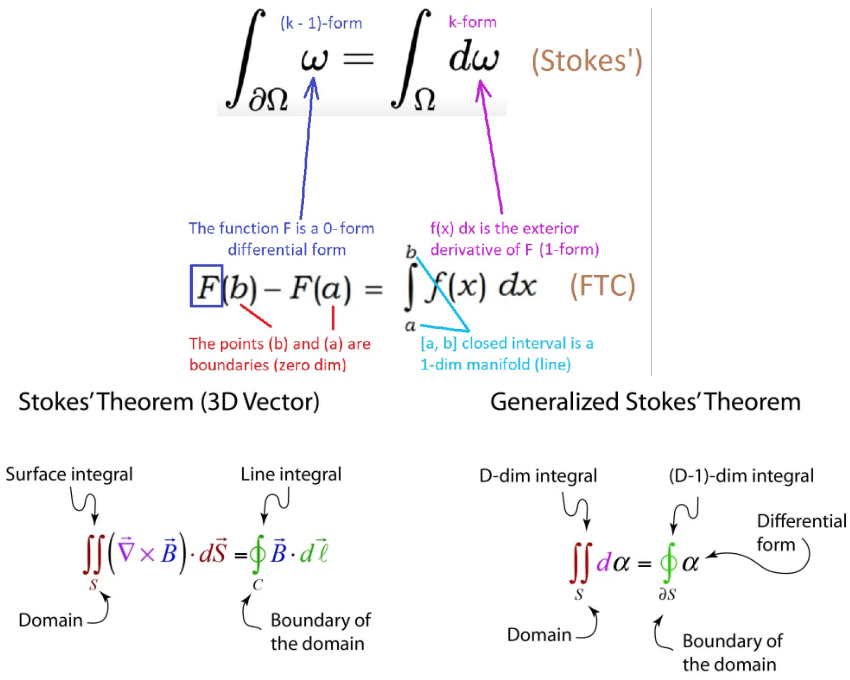
Stokes’ Theorem : \(\oint_Sds\vec{F}\cdot\hat{t}=\int_SdS(\nabla\times\vec{F})\cdot\hat{n}\) or that the line integral around the path and the surface integral over the area bounded by the path is related 1:1.
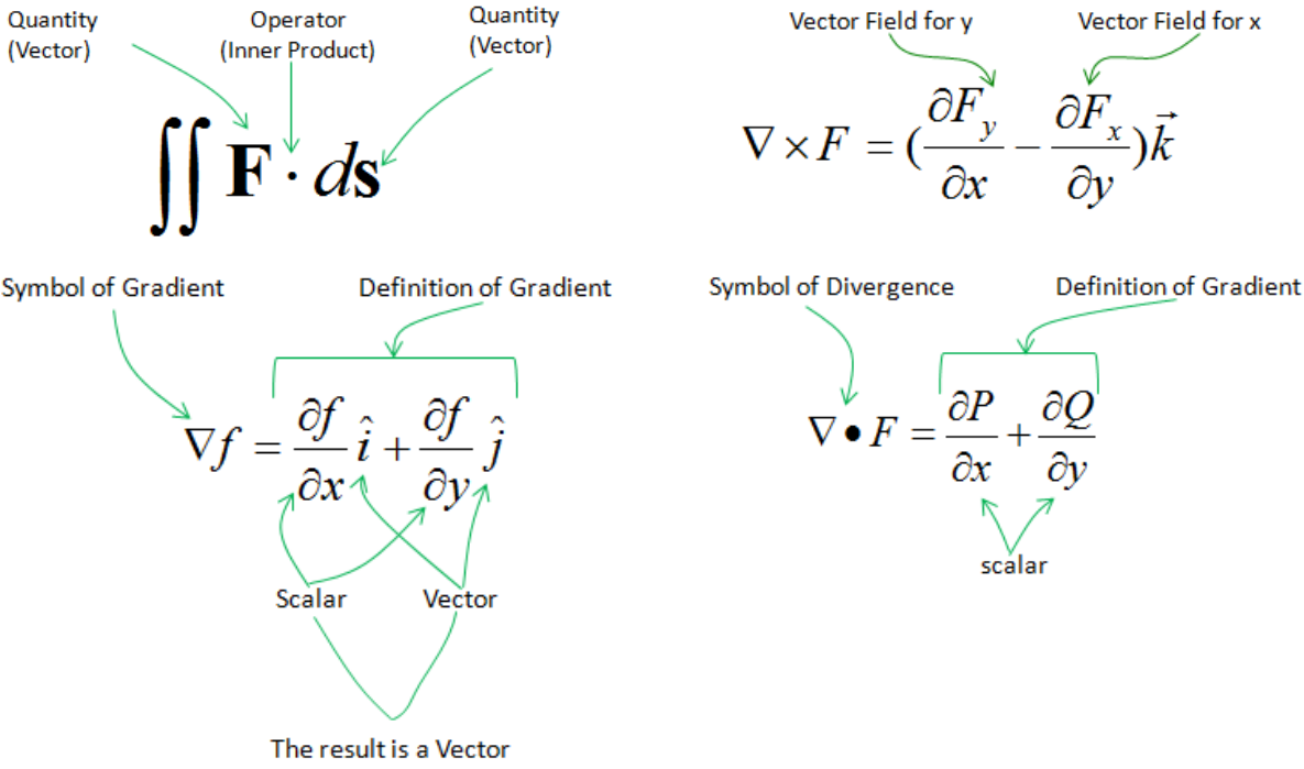
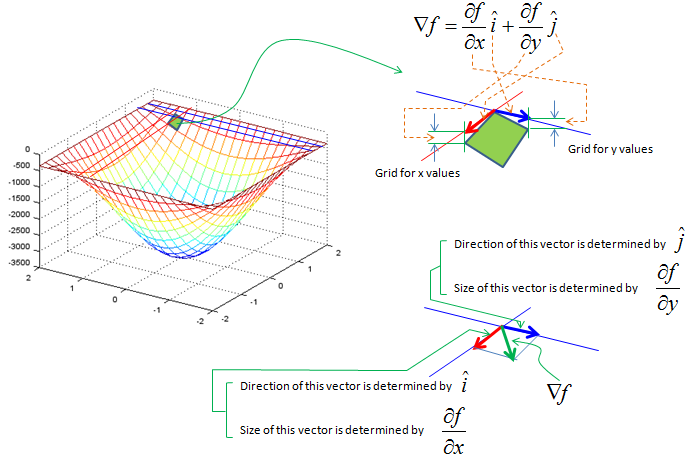
Gradient(\(\nabla f\)):
Cartesian Coordinates : \(\nabla f=\frac{\partial f}{\partial x}\hat{i}+\frac{\partial f}{\partial y}\hat{j}+\frac{\partial f}{\partial z}\hat{k}\)
Polar/Cylindrical Coordinates : \(\nabla f=\frac{df}{dr}\hat{r}+\frac{1}{r}\frac{df}{d\theta}\hat{\theta}+\frac{df}{dz}\hat{z}\)
Spherical Coordinates : \(\nabla f=\frac{df}{dr}\hat{r}+\frac{1}{r}\frac{df}{d\theta}\hat{\theta}+\frac{1}{r\sin{\theta}}\frac{df}{d\phi}\hat{\phi}\)
Generalized Stokes’ theorem or Fundamental Theorem of Multivariate Calculus
In case you are curious, this deeper theorem captures all above theorems (and more) in one formula,
by analysing differential forms on manifolds, which simplifies several theorems from vector calculus
13.3.2. Coding review#
var('r')
f=cos(y)*(x-r^3/x^2)
s(diff(f,x))
s(diff(f,y)/x)
var('r E v')
f=cos(y)*(x*E+(r^2*(v-E*r))/x^2)
s(diff(f,x))
s(diff(f,y)/x)
s(diff(f,z)/(r*sin(y)))
SageManifolds solve differential geometry and tensor calculus of any dimension
# vector field - div, curl
E.<x,y,z> = EuclideanSpace()  # set up coordinates in ()
v = E.vector_field(x^2-y^2, -2*x*y, 0, name='v')
sca = E.scalar_field(x^2+y^2-z^2, name='sca')
s(v.display()) # original func
s(sca.display())

s(v.div().display())
s(v.curl().display())
from sage.manifolds.operators import grad, laplacian
s(grad(sca).display())
s(laplacian(sca).display())
# divergence algo (manually)
var('x y z') ; Fx=z^2 ; Fy=x^2 ; Fz=-y^2
div = diff(Fx,x) + diff(Fy,y) + diff(Fz,z)
s(div)

# curl Approach 1: self-made algorithm
curlx = diff(Fz,y) - diff(Fy,z)
curly = diff(Fx,z) - diff(Fz,x)
curlz = diff(Fy,x) - diff(Fx,y)
s(vector([curlx, curly, curlz]))

# curl Approach 2: built-in function
E.<x,y,z> = EuclideanSpace()
v = E.vector_field(z^2, x^2, -y^2, name='v')
s(v.curl().display())

E = EuclideanSpace(3)  # btw: set up
s(E.cartesian_coordinates())
s(E.cylindrical_coordinates())
s(E.spherical_coordinates())
# From vector to calculus
v = vector(RR, [1.2, 3.5, 4.6])
w = vector(RR, [1.7,-2.3,5.2])
s(v*w)
s(v.cross_product(w))

# Vector Calculus
var('t')
r=vector((2*t-4, t^2, (1/4)*t^3)) # start from displacement formula
s(r)
s(r(t=5))

velocity = r.diff(t) # now velocity formula
s(velocity)       # this expression does not function as a function
s(velocity(t=1))  # so we substitute explicitly
T=velocity/velocity.norm() # calculate the unit vector
s(T(t=1).n())
arc_length = numerical_integral(velocity.norm(), 0,1)
s(arc_length)
x,y,z=var('x y z')
plot_vector_field3d((x*cos(z),-y*cos(z),sin(z)), (x,0,pi), (y,0,pi), (z,0,pi),colors=['red','green','blue'])
13.3.3. Week 6#
var('y')
s(diff((ln(x^2+y^2))/2,y))
s(diff(arctan(y/x),x))
s(n(arctan(3+sqrt(3))*180/pi))
s(n(sqrt(13+6*sqrt(3))))
13.3.4. Week 5#
var('y a n')
f=a*e^(-x-y-a)
s(integral(integral(f,x,0,a),y,0,a))
s(diff(-x*y/(x^2+y^2),x))
s(diff(x^2/(x^2+y^2),y))
s(diff(1/(x^2+1)^(3/2),x))
s(expand(integral(3*x*(y-(a/2)),x,n-(a/2),n+(a/2))))
13.3.5. Week 4#
var('x y')
s(diff(x/sqrt(x^2+y^2), y))
s(diff(y/sqrt(x^2+y^2), x))
s(diff(-x/sqrt(x^2+y^2), x))
s(diff(-y/sqrt(x^2+y^2), y))
13.4. Complex Analysis#
Notes:
Cauchy-Riemann Equations(\(z=x+iv\)): \(\frac{du}{dx}=\frac{dv}{dy}\quad\frac{du}{dy}=-\frac{dv}{dx}\)
Rewritten Form: \(\frac{du}{dx}-\frac{dv}{dy}=0\quad\frac{du}{dy}+\frac{dv}{dx}=0\)
Any function that satisfies these equations are analytic.
(Cauchy’s) Residue Theorem: \(\int_\gamma dzg(z)=2\pi i\sum_{\text{poles of g inside }\gamma}(\text{residue of each pole of }g)\)
Residue: The residue of f(z) is \(\lim_{z\rightarrow z_0}f(z)(z-z_0)\). It can \(\lim_{z\rightarrow z_n}(z-z_n)(\text{integrand of contour integral})\)
13.4.1. Coding review#
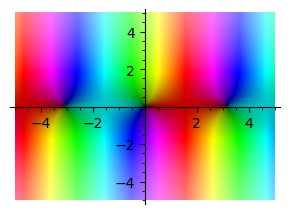
show(complex_plot(sin(x), (-5, 5), (-5, 5), figsize=3))
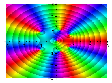
f(z)=z^5 + z - 1 + 1/z
complex_plot(f, (-3, 3), (-3, 3), plot_points=300,figsize=4,contoured=True)
13.4.2. Week 8#
limit(pi*cot(pi*z)/z^2,z=0)
Infinity
var('a b')
assume(a>0)
assume(b>0)
bool(integral(cos(b*x)/(x^2+a^2),x,-oo,oo)==pi*(e^(-a*b))/a)
True
var('u b')
s(diff((x-u)*e^(i*b*x),x))
bool(integral(1/(2-sin(x)),x,0,2*pi)==2*pi/sqrt(3))
var('a')
assume(a>0)
assume(a<1)
integral(1/(1+a^2-2*a*cos(x)),x,0,2*pi)
s(diff((x-u)*e^(i*m*x),x))
assume(m>0)
s(integral(cos(m*x)/(1+x^4),x,0,oo))
var('u')
s((1-u/2+u^2/24)/(1-u/6+u^2/120))
s(diff(tan(pi*x),x))
s(diff((x-u)*cos(pi*x),x))
s(diff(cot(pi*x),x))
s(diff(sin(pi*x)^2))
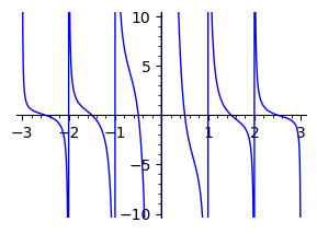
plot(pi/(x^2*tan(pi*x)),x,-3,3,ymin=-10,ymax=10,figsize=3)
var('c y z')
f=x^y*cos(z)
s(diff(x^2*diff(f,x),x)+diff(sin(z)*diff(f,z),z)/sin(z))
s(integral(1/(x^2-2*x+4),x,-oo,oo))
s(diff(x^2*tan(pi*x),x))
s(diff(pi*cot(pi*x),x))
s(diff(x^2/(pi*cot(pi*x)),x))
var('x y')
z=x+i*y
print(bool(1/z==(x-i*y)/(x^2+y^2)))
print(bool(z^2==x^2-y^2+2*i*x*y))
print(bool(z^3==x*(x^2-3*y^2)+i*y*(3*x^2-y^2)))
var('x')
print(n(integral( (x+2-i) / (x-3*i/2) ,x,-1,1)/2/pi/i))
print(n(integral(i*(1+i*x+2)/(1+i*x-i/2),x,-1,1)/2/pi/i))
print(n(integral((x-i-2)/(-x+i-i/2),x,-1,1)/2/pi/i))
print(n(integral(i*(1-i*x)/(i*x+1+i/2),x,-1,1)/2/pi/i))
0.374334083621998 - 0.224726365278291*I
0.740707869608976 + 0.267178513616855*I
0.704832764699133 + 0.494518077358574*I
0.180125282069893 - 0.0369702256971377*I
13.5. Linear Algebra#
13.5.1. Review#
Algebra |
Linear Algebra |
Concept consistency |
|---|---|---|
Solves scalar equations, e.g., polynomials like \(ax^2+bx+c=0\). Methods: factoring, quadratic formula. |
Solves systems of linear equations, e.g., \(Ax=b\). Methods: Gaussian elimination, matrix inversion. |
Solving Equations: Both seek solutions to equations; algebra focuses on scalar polynomials, linear algebra on vector/matrix systems. |
Finds roots of polynomials, e.g., \(x^2 - 3x + 2 = 0\) gives \(x=1,2\). |
Finds eigenvalues via characteristic polynomial \(\det(A - \lambda I) = 0\) . |
Roots and Eigenvalues: Both involve root-finding of polynomials; eigenvalues are roots of matrix-derived polynomials. |
Operations on numbers, polynomials, or abstract structures (groups, rings). E.g., polynomial multiplication. |
Operations on vectors/matrices (addition, multiplication). Vector spaces define structure. |
Operations and Structures: Both study structured sets with operations; algebra emphasizes general algebraic structures, linear algebra focuses on vector spaces. |
Studies functions, e.g., \(f(x) = x^2 + 3\), or homomorphisms in abstract algebra. |
Studies linear transformations, e.g., \(T(v) = Av\), represented by matrices. |
Functions and Transformations: Both analyze mappings; algebra includes nonlinear functions, linear algebra restricts to linear transformations. |
Factors polynomials, e.g., \(x^2 - 1 = (x-1)(x+1)\), or integers into primes. |
Decomposes matrices, e.g., eigendecomposition \(A = PDP^{-1}\) or LU decomposition. |
Factorization and Decomposition: Both break complex objects into simpler parts; algebra factors scalars, linear algebra decomposes matrices. |
Studies groups, rings, fields. E.g., integers form a ring, polynomials a ring. |
Studies vector spaces, matrix rings. E.g., \(n \times n\) matrices form a ring. |
Abstract Structures: Both explore abstract systems with operations; vector spaces are modules, and matrix rings align with algebraic rings. |
Notes
Row Reduction : Method where make lower-left triangle of 0s using augmentation. Uses shown below.
Linear Equations(Homogeneous : all RHS’s=0) : Solve for variables one by one.
Determinant : Product of the lead diagonal as all other products will be 0.
Inverse : Use augmentation to find inverse.
Inverse(\(AA^{-1}=I\)) : Use cofactors and adjoint(or row reduction) then divide by determinant(can also calculate using row reduction).
Determinant : Measures the factor by which an area or volume is multiplied by. Calculate using formula or row reduction.
Gram-Schmidt Orthogonalization :
Formula:
\(\large\hat{e_1}=\frac{v_1}{\sqrt{v_1\cdot v_1}}\)
\(\large\hat{e_2}=\frac{v_2-(v_2\cdot\hat{e_1})\hat{e_1}}{|\vec{e_2}|}\)
\(\large\hat{e_3}=\frac{v_3-(v_3\cdot\hat{e_1})\hat{e_1}-(v_3\cdot\hat{e_2})\hat{e_2}}{|\vec{e_3}|}\)
For orthogonalization, determine coefficients by using the fact that \((e_i\cdot e_j)=0\) where \(\cdot\) can mean dot product of \((f\cdot g)=\int_0^1dxf(x)g(x)\)
Applications : Includes linear algebra, numerical analysis, quantum mechanics, machine learning etc.
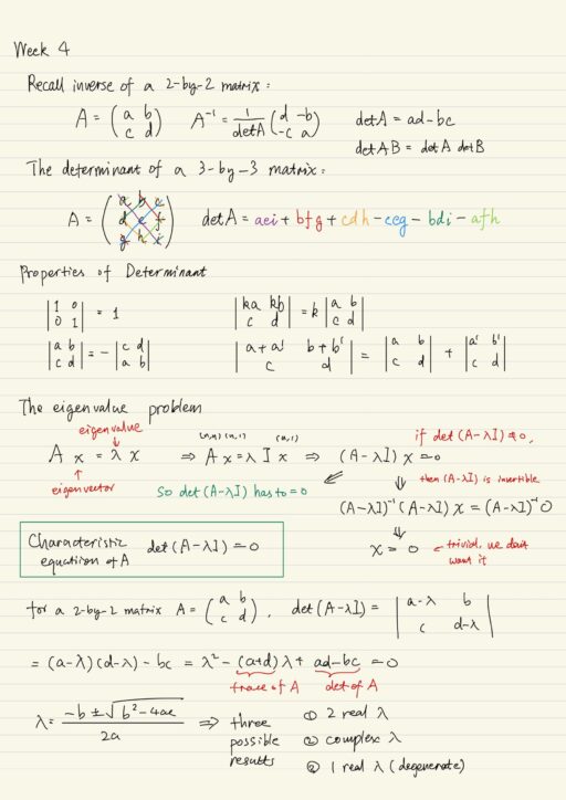
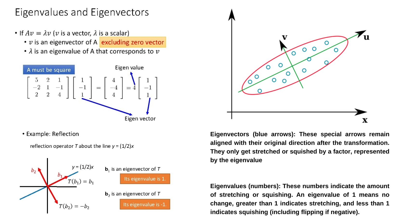
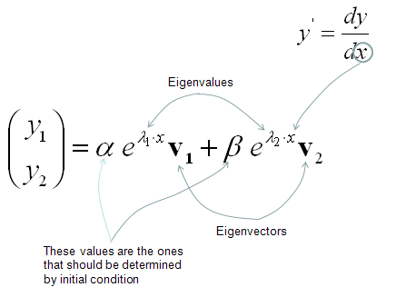
Eigenvalues & Eigenvectors
Use determinant formula : Determinant of matrix minus \(\lambda I=0\)
Quick Method :
The mean of the eigenvalues is the mean of the numbers on the lead diagonal.
The determinant of the matrix is the product of the eigenvalues.
\(d^2=m^2-p\) Eigenvalues \(= m\pm d\)
Lab Notes
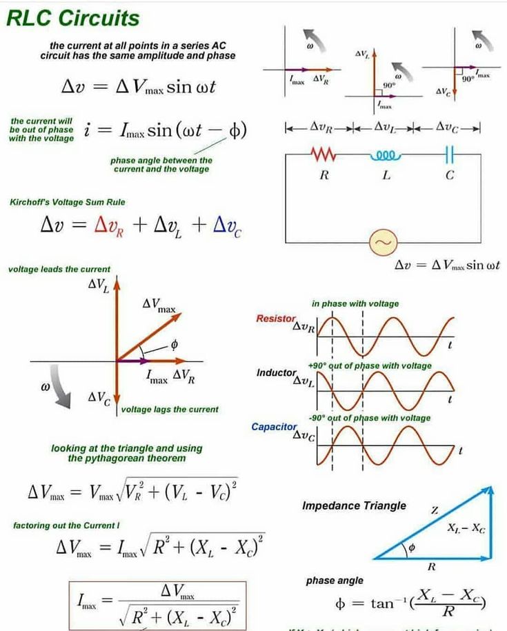
When in series(circuit), the current is always the same.
Kirchhoff’s Laws(can be used to solve for current or voltage)
Current Law : The current entering a node is the same as the current exiting the same node as electrons can be created out of nothing and can’t just disappear.
Voltage Law : The voltage drop is 0 (one of the capacitors or resistors will probably be a voltage gain.)
Types of Circuits :
Series
Parallel
RC(R:resistor, C:capacitor) : Circuit that comprises of only resistors and capacitors(and stuff connecting them). This has a constant current as it is only affected using arithmetic operations by the resistors and capacitors.
RL/RLC(L:Inductor) : Circuit that also has an inductor which causes a non-constant current(\(V_L=L\frac{dI}{dt}\)).
RLC circuits can make microwaves oscillating at its resonant frequency. Then using formulae you can get the right wavelength using the formula to make microwaves.
diff btw C and L??
13.5.2. Problem Set 11#
f(x) = 20*x^4-85*x^3-8037/16*x^2+5231/16*x+33789/128
f(5/4)
# Define the polynomials
R.<x> = QQ[] # Polynomial ring for rational field
f = 20*x^4-85*x^3-8037/16*x^2+5231/16*x+33789/128
g = 2*x - 5

# Perform long division using quo_rem()
q, r = f.quo_rem(g)  # q is the quotient, r is the remainder

# Print the results
s(f"Quotient: {q}")
s(f"Remainder: {r}")
a=8*x^4-90*x^3-5089/16*x^2+61009/128
b=4*x^3+71/2*x^2-104*x+3211/32
c=x^2-13/2*x+185/16
s(expand(a+b*(2*x-5)+c*(2*x-5)^2))
a=y*(13/4-x)-(8*x^2*y-45*x*y+247/4*y)/(20-8*x)
b=(8*x^2*y-45*x*y+247/4*y)/(20-8*x)
s(expand(a^2+y^2+b^2)) # x=lambda
var('x y z')
s(expand((19-8*x)*(y*(13/4-x)-z)))
var('a b d')
A=matrix(2,2,[a,b,b,d])
m=A.trace()/2
p=A.det()
l=m-sqrt(m^2-p)
s(a-l,d-l)
13.5.3. Week 10#
var('k l m1 m2 w')
A=matrix(2,2,[w^2-(k+l)/m1,l/m1,l/m2,w^2-(k+l)/m2])
s(A.eigenvalues())
var('a b c')
s(expand((2*x-1)*(a+b*x+c*x^2)))
s(integral((a+b*x+c*x^2)^2,x,0,1))
s(integral(a*x^2+b*x+c,x,-1,1))
s(integral(x*(a*x^2+b*x+c),x,-1,1))
s(integral((a*x^2+c)^2,x,-1,1))
A=matrix([[2,1,-sqrt(2)]
        ,[1,1,sqrt(2)]
        ,[-sqrt(2),sqrt(2),1]])
s(expand(A.det()))
s(A.eigenvectors_right())
Row Reduction
M=[[1,0,0,6,2],[7,5,3,3,5],[3,1,4,3,4],[8,0,0,0,2],[5,8,3,5,7]] # input matrix
for i in [1,2,3,4]: # for 2nd to 5th rows
    for j in [1,2,3,4]: # for 2nd to 5th columns
        M[i][j]-=M[0][j]*M[i][0]/M[0][0] # minus the number required
    M[i][0]=0 # change number in 1st column to 0
for i in [2,3,4]: # repeat process
    for j in [2,3,4]:
        M[i][j]-=M[1][j]*M[i][1]/M[1][1]
    M[i][1]=0
for i in [3,4]:
    for j in [3,4]:
        M[i][j]-=M[2][j]*M[i][2]/M[2][2]
    M[i][2]=0
M[4][4]-=M[3][4]*M[4][3]/M[3][3]
M[4][3]=0
s(matrix(5,5,M))
s(factor(10062))
s(factor(75335))
s(factor(31434))
s(factor(80002))
s(factor(58357))
s(factor(408))
13.5.4. Week 9#
var('t')
assume(t>0)
bool(integral(e^(i*t*x)/(x-3-i),x,-oo,oo)==2*pi*i*e^(-t+3*i*t))
A=matrix(4,4,[1,3,-1,2,2,1,3,1,-1,2,-4,1,-2,1,2,-3])
A.det()
0
var('x')
A=matrix(3,3,[1,2-x^2,2,2,3,1,2,3,1])
A.det()
expand(-3*(2-x^2)*(9-x^2)+3*(9-x^2)+15*(2-x^2)-15)
-3*x^4 + 15*x^2 - 12
13.6. Differential Equations & Fourier Analysis#
13.6.1. Review#
Notes:
For a first-order DE, \(\frac{dy(t)}{dt}+q(t)y(t)=r(t)\text{ has a solution }y(t)=y(t_0)e^{-\int_{t_0}^t q(t')dt'}+e^{-\int_{t_0}^t q(t''')dt'''}\int_{t_0}^t dt'\,r(t') e^{\int_{t_0}^{t'}dt'' q(t'')}\)
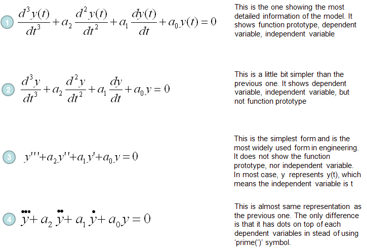
\(y(t)\) Function Prototype, \(t\) Dependent Variable
\(y\) Function Name = Independent Variable Five Easy Pieces(Non-linear ODE)
For non-linear ODE of the form \(N(t,y)dy+M(t,y)dt=0\) use five easy pieces.
If it is of the form \(\frac{dy}{dt}+q(t)y=r(t)y^n\) then substitute \(w=y^{1-n}\)
Is it of the form \(N(y)\text{ and }M(t)\)? Then directly integrate
Are both \(M\) and \(N\) homogeneous of the same degree(This means that \(M(\lambda t,\lambda y)=\lambda^kM(t,y)\) and \(N(\lambda t,\lambda y)=\lambda^k N(t,y)\).)? Reduce equation to 2nd form.
Is it an exact differential : Check \(\frac{\partial M}{\partial y}=\frac{\partial N}{\partial t}\). If yes, find a function \(F\) such that it is an exact differential when integrating \(M\) and \(N\) to \(t\) and \(y\) respectively. Add the appropriate \(+C\) to make the form work.
Is it reducible to exact? Check by \(\frac{1}{N}\left ( \frac{\partial M}{\partial y}-\frac{\partial N}{\partial t}\right )\) and \(\frac{1}{M}\left ( \frac{\partial M}{\partial y}-\frac{\partial N}{\partial t}\right )\). \(Q = \exp \left[ {\int} \frac{1}{M} \left( \frac{\partial N}{\partial t}-\frac{\partial M}{\partial y} \right) dy \right]\)
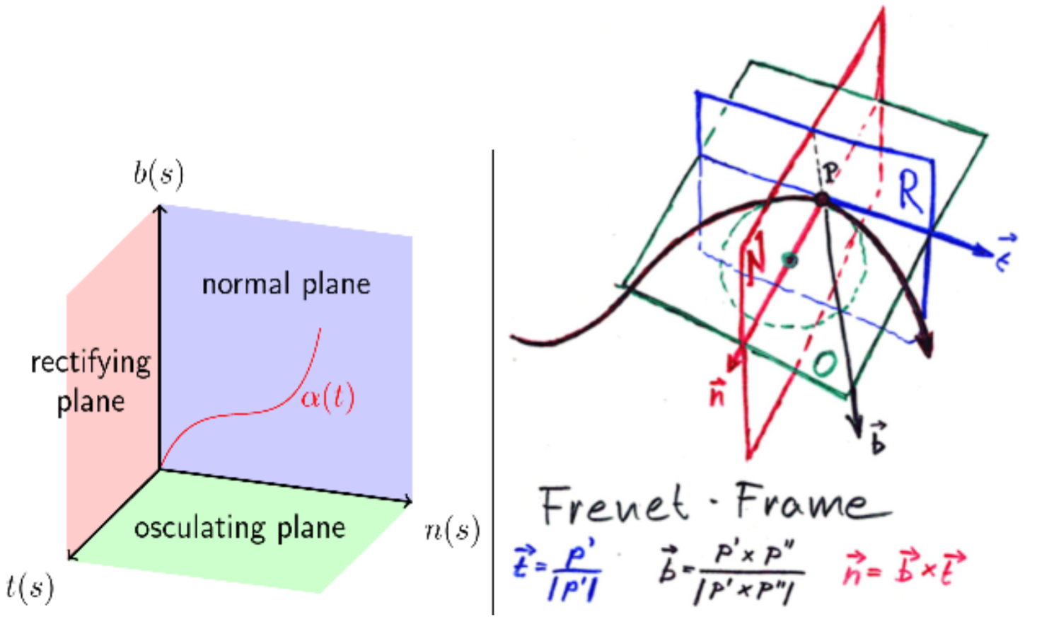
Frenet-Serret Apparatus
Tangent : \(\vec{T}=\frac{d\alpha(s)}{ds}\)
Normal Vector & Curvature : \(\frac{d\vec{T}}{ds}=N(s)\kappa(s)\) & \(|N(s)|=1\)
Binormal Vector & Torsion : \(\vec{B}=\vec{T}\times\vec{N}\) & \(\tau(s)=-\frac{d\vec{B}}{ds}\cdot\vec{N}\)
notations:
Four categories: order, linear, homo, PDE
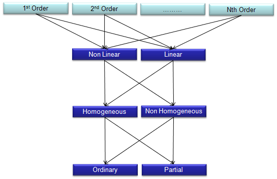
n-order 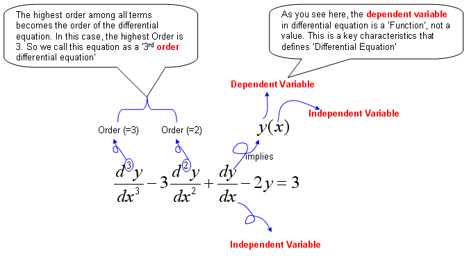
Homo VS. Non-Homo 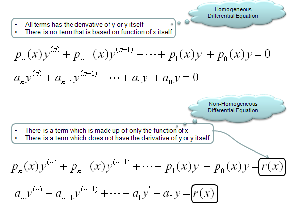
PDE 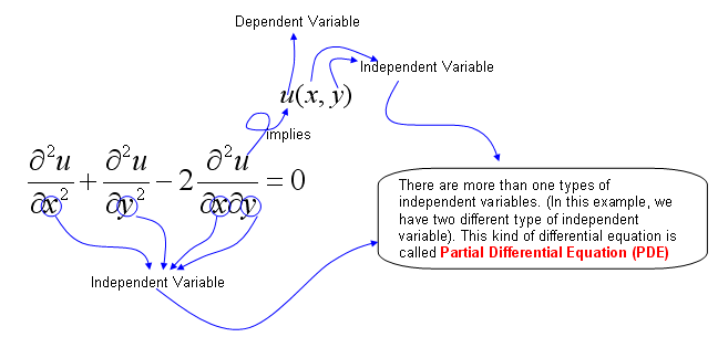
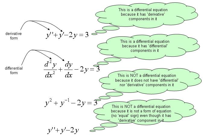
DE is governing equation
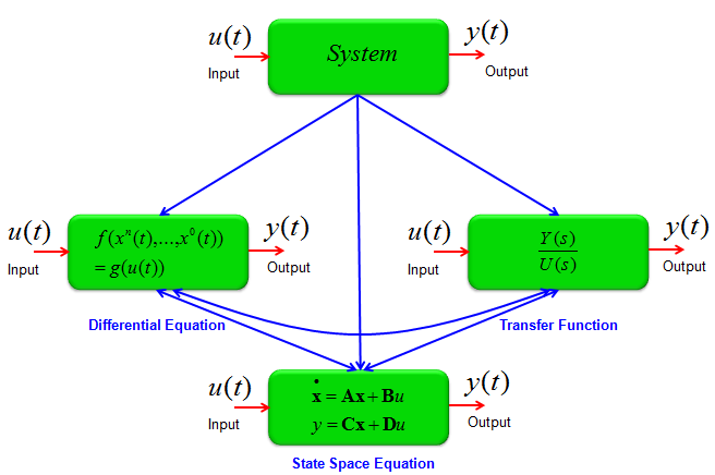
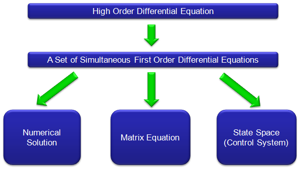
Converting High Order Differential Equation into First Order Simultaneous Differential Equation
e.g. 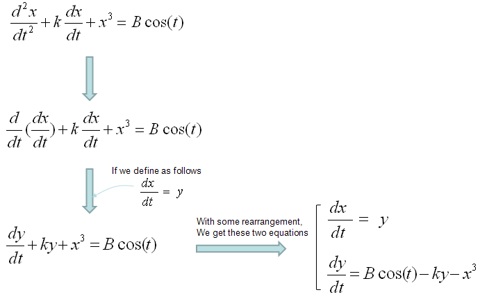
Common Types of DE
Separable differential equations
First-order linear differential equations
Simple Harmonic Motion
Homogeneous linear differential equations with constant coefficients
Bernoulli’s equation
Logistic differential equations
Systmes of linear differential equations
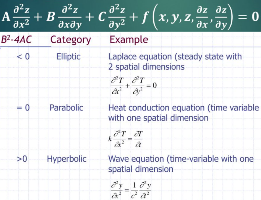
Types of PDE
Wu–Yang dictionary links concepts in particle physics (specifically gauge theory) and mathematics (differential geometry and fiber bundle theory)
Particle Physics Term |
Mathematical Term |
Description |
|---|---|---|
Gauge Field |
Connection on a Fiber Bundle |
The gauge field, which describes interactions in gauge theories (e.g., electromagnetic or Yang-Mills fields), corresponds to a connection on a principal fiber bundle, defining how fields transform across space-time. |
Gauge Potential (e.g., \(A_\mu\)) |
Connection Form |
The gauge potential, a vector potential like the electromagnetic potential, is mathematically represented as a connection form, a differential form that encodes the connection on the bundle. |
Field Strength (e.g., \(F_{\mu\nu}\)) |
Curvature of the Connection |
The field strength tensor, which quantifies the strength of the gauge field (e.g., electromagnetic field tensor), corresponds to the curvature of the connection, a 2-form derived from the connection form. |
Gauge Transformation |
Change of Local Trivialization (or Section) |
A gauge transformation, which adjusts the gauge potential to describe the same physical situation, is equivalent to changing the local trivialization or section of the fiber bundle, altering the coordinate system without changing the bundle’s structure. |
Source (e.g., Electric Current) |
(No Direct Equivalent) |
In the original Wu-Yang dictionary, sources like electric currents were included but lacked a direct mathematical analogue, indicating a gap in the correspondence at the time. This later inspired mathematical developments, such as Donaldson theory. |
Phase Factor (Nonintegrable) |
Holonomy |
The nonintegrable phase factor, as seen in phenomena like the Aharonov-Bohm effect, corresponds to holonomy, which describes the geometric phase acquired by a vector transported around a closed loop on the bundle. |
Magnetic Monopole |
Nontrivial Fiber Bundle |
The magnetic monopole, such as the Wu-Yang monopole, is described by a nontrivial fiber bundle, where the bundle’s topology (e.g., Hopf fibration) prevents a global gauge choice, explaining quantization conditions. |
Aspect |
Classical Mechanics |
Quantum Mechanics |
|---|---|---|
Definition |
Describes the motion of macroscopic objects using Newton’s laws and deterministic principles. |
Governs the behavior of particles at atomic and subatomic scales using probabilistic principles. |
Scale |
Macroscopic (e.g., planets, cars, projectiles). |
Microscopic (e.g., atoms, electrons, photons). |
Nature of Motion |
Deterministic: Future states can be precisely predicted given initial conditions. |
Probabilistic: Outcomes are described by probabilities (wave functions). |
Key Principles |
- Newton’s Laws of Motion |
- Wave-particle duality |
Position and Momentum |
Can be measured simultaneously with arbitrary precision. |
Subject to Heisenberg’s Uncertainty Principle (cannot measure both precisely at once). |
Energy |
Continuous energy levels. |
Quantized energy levels (discrete values). |
Wave-Particle Duality |
Objects are either particles or waves, not both. |
Particles exhibit both wave-like and particle-like properties (e.g., electrons, light). |
Mathematical Framework |
Uses differential equations (e.g., F = ma). |
Uses wave functions, Schrödinger equation, and matrix mechanics. |
Measurement |
Measurement does not affect the system’s state. |
Measurement collapses the wave function, altering the system’s state. |
Superposition |
Not applicable; objects exist in one definite state. |
Particles exist in multiple states simultaneously until measured. |
Entanglement |
Not applicable. |
Quantum systems can be entangled, sharing special correlations regardless of distance. |
Examples of Phenomena |
- Planetary orbits |
- Electron orbitals in atoms |
Key Figures |
Isaac Newton, Lagrange, Hamilton |
Max Planck, Werner Heisenberg, Erwin Schrödinger, Niels Bohr |
Applications |
Engineering, astronomy, mechanics of everyday objects. |
Quantum computing, semiconductors, lasers, MRI, atomic clocks. |
Limitations |
Fails at very small scales or high speeds (near the speed of light). |
Complex calculations; less intuitive for macroscopic systems. |
Five quantum behaviours:
Wave-particle duality: Tiny particles look like they are behaving like waves or particles, depending on how you observe them.
Superposition: In the quantum world, particles can exist in multiple states at once.
The Heisenberg uncertainty principle: Nature imposes a fundamental limit on how precisely you can measure something. (You can’t measure certain pairs of properties at the same time with unlimited precision.)
Entanglement: Two things can be so interconnected that they influence each other, regardless of distance apart.
Spin: Spin is a fundamental characteristic of elementary particles. Like mass or charge, spin determines a particle’s behavior and interaction with other particles.
Further comparison btw Classical and Quantum in terms of Math
Aspect |
Classical Mechanics |
Quantum Mechanics |
|---|---|---|
Core Mathematical Framework |
Newtonian mechanics, Lagrangian, or Hamiltonian formulations with differential equations. |
Wave functions, operators, and matrix mechanics, governed by the Schrödinger equation. |
Key Equations |
- Newton’s Second Law: \( F = ma \) |
- Time-dependent Schrödinger Equation: \( i\hbar \frac{\partial \psi}{\partial t} = \hat{H}\psi \) |
Variables |
Position (\( x \)), velocity (\( v \)), acceleration (\( a \)), momentum (\( p = mv \)). |
Wave function (\( \psi \)), probability density (\(\mid \psi \mid^2\)). |
Nature of Variables |
Continuous and deterministic. |
Probabilistic; wave function describes probability amplitudes. |
Mathematical Tools |
- Ordinary differential equations (ODEs) |
- Partial differential equations (PDEs) |
State Representation |
Precise coordinates in phase space (position and momentum). |
Wave function \( \psi(x,t) \) in a complex Hilbert space. |
Time Evolution |
Deterministic via Newton’s laws or Hamilton’s equations. |
Probabilistic via the Schrödinger equation. |
Operators |
Not used; variables are directly measurable. |
Observables are Hermitian operators (e.g., position \( \hat{x} \), momentum \( \hat{p} \)). |
Commutation Relations |
Variables commute (e.g., \( xp = px \)). |
Non-commutative operators, e.g., \( [\hat{x}, \hat{p}] = i\hbar \). |
Energy Representation |
Energy as a scalar: \( E = T + V \). |
Energy via Hamiltonian operator: \( \hat{H}\psi = E\psi \). |
Probability |
Not probabilistic; motion is fully predictable. |
Probabilistic; probability density given by \( \mid \psi \mid^2 \). |
Quantization |
Continuous variables (energy, position, etc.). |
Quantized observables (e.g., discrete energy levels). |
Boundary Conditions |
Define specific solutions to differential equations. |
Constrain wave function (e.g., normalization, continuity). |
Examples of Calculations |
- Projectile trajectory: \( x(t) = x_0 + v_0 t + \frac{1}{2} a t^2 \) |
- Hydrogen atom energy levels: \( E_n = -\frac{13.6}{n^2} \) eV |
Coordinate System |
Cartesian or generalized coordinates in configuration space. |
Abstract Hilbert space or position/momentum representations. |
Complex Numbers |
Rarely used; real-valued quantities dominate. |
Essential; wave functions are complex-valued. |
13.6.2. Week 13#
s(diff(e^t*cos(2*t),t))
s(diff(e^t*sin(2*t),t))
print(bool(diff(B,t,2)-2*diff(B,t)+5*B==t*e^t*sin(2*t)))
A(t)=diff(B,t)
B(t)=B
B(0)
C=B-e^t*cos(2*t)/64+e^t*sin(2*t)/2
print(bool(diff(C,t,2)-2*diff(C,t)+5*C==t*e^t*sin(2*t)))
A=e^t/64*(cos(2*t)*(1-8*t^2)+4*t*sin(2*t)-cos(2*t)-32*sin(2*t))
B=e^t*(cos(2*t)*(t*sin(4*t)/16+cos(4*t)/64-t^2/8)+sin(2*t)*(sin(4*t)/64-t*cos(4*t)/16))
s(B)
bool(A==B)
False
y=e^t/64*(cos(2*t)*(1-8*t^2)+4*t*sin(2*t)-cos(2*t)-32*sin(2*t))
bool(diff(y,t,2)-2*diff(y,t)+5*y==t*e^t*sin(2*t))
y=function('y')(t)
s(desolve(diff(y,t,2)-2*diff(y,t)+5*y==t*e^t*sin(2*t),y,ics=[0,0,1],show_method=True))
var('t')
print(bool(e^t/64*(cos(2*t)*(1-8*t^2)+4*t*sin(2*t))==e^t*(cos(2*t)*(t*sin(4*t)/16+cos(4*t)/64-t^2/8)+sin(2*t)*(sin(4*t)/64-t*cos(4*t)/16))))
s(diff(e^t/64*(cos(2*t)*(1-8*t^2)+4*t*sin(2*t)),t))
True
var('t E_0 omega_0 R L C')
s(diff(E_0/(i*R*omega_0-L*omega_0^2+1/C)*e^(i*omega_0*t),t))
var('y10 y11 y12 y20 y21 y22 y30 y31 y32')
var('a2 a1 a0')
y13=-(a2*y12+a1*y11+a0*y10)
y23=-(a2*y22+a1*y21+a0*y20)
y33=-(a2*y32+a1*y31+a0*y30)
A=matrix(3,3,[y11,y21,y31,y11,y21,y31,y12,y22,y32])
C=matrix(3,3,[y10,y20,y30,y12,y22,y32,y12,y22,y32])
E=matrix(3,3,[y10,y20,y30,y11,y21,y31,y13,y23,y33])
B=E.det()
W=matrix(3,3,[y10,y20,y30,y11,y21,y31,y12,y22,y32])
W1=W.det()
s(expand(B))
s(expand(W1))
var('t')
s(diff(e^t*(cos(2*t)*(t*sin(4*t)/16+cos(4*t)/64-t^2/8)+sin(2*t)*(sin(4*t)/64-t*cos(4*t)/16)),t))
s(integral(x*sin(2*x)/2,x))
s(integral(x*sin(2*x)*cos(2*x)/2,x))
A2=x*sin(2*x)*cos(2*x)/2
A1=-A2*sin(2*x)/cos(2*x)
s(A1,A2)
print(bool(A1==-x*sin(2*x)*sin(4*x)/4/cos(2*x)))
A1=integral(A1,x)
A2=integral(A2,x)
s(A1,A2)
True
s(expand(A[1][1]))
A=[[cos(2*x),sin(2*x)],[cos(2*x)-2*sin(2*x),sin(2*x)+2*cos(2*x)]]
A[1][1]-=A[0][1]*A[1][0]/A[0][0]
A[1][0]=0
s(matrix(A))
s(diff(e^x*cos(2*x),x))
s(diff(e^x*sin(2*x),x))
f(x)=4*x^4+28*x^3+81*x^2+112*x+64
g(x)=x+2
f.maxima_methods().divide(g)
[4*x^3 + 20*x^2 + 41*x + 30, 4]
s(expand((1/(2*sqrt(x^2/2+1)-x^2/(4*(x^2/2+1)^(3/2))))^2))
s(expand((x/(x^2/2+1)^(3/2))^2))
s(expand(x^4+(4*x^2+8)*(x^2+2)^3-4*x^2*(x^2+2)^2))
s(sqrt(2/(2+x^2)))
A=vector([sqrt(2)/(2+x^2)^(3/2),0,-x/(2+x^2)^(3/2)])
s(A)
B=vector([sqrt(2)/sqrt(2+x^2),0,-x/sqrt(2+x^2)])
s(A.dot_product(B))
bool(2/(2+x^2)+x^2/(x^2+2)^2==(4+3*x^2)/(2+x^2)^2)
True
A=vector([sqrt(2)/(2+x^2)^(3/2),0,-x/(2+x^2)^(3/2)])
B=vector([-x/sqrt(2*(2+x^2)),1/sqrt(2),-1/sqrt(2+x^2)])
s(-diff(B,x))
s(A)
bool(A==-diff(B,x))
False
s(diff(1/sqrt(2+x^2),x))
s(diff(x/sqrt(2*(2+x^2))))
A=vector([sqrt(1+x^2/2),x/sqrt(2),arcsinh(x/sqrt(2))]) # alpha(s)
T=diff(A,x) # calculate tangent vector
N1=diff(T,x) # calculate normal vector times curvature
s(N1)
s(simplify(N1.norm())) # calculate curvature (magnitude of unnormalized normal vector
N=N1/N1.norm() # normalize normal vector
B=vector([-2*x/sqrt(x^2+1),x^2/(x^2+1)+1/(x^2+1)^(3/2),-2/sqrt(x^2+1)])
s(diff(B,x))
s(N)
T=vector([x/sqrt(x^2+1),2,1/(x^2+1)])
N=vector([1/sqrt(x^2+1),0,-x/sqrt(1+x^2)])
s(T.cross_product(N))
s(expand(x^2-2*x^2*(x^2+1)+x^4+(x^2+1)^3))
s(expand(diff(x/sqrt(x^2+1),x)^2+diff(1/sqrt(x^2+1),x)^2))
s(diff(x/sqrt(x^2+1),x))
s(diff(1/sqrt(x^2+1),x))
s(diff(sqrt(1+x^2),x))
s(diff(2*x,x))
s(diff(ln(x+sqrt(1+x^2))))
bool(x^2/(x^2+1)+4+(x^2/(x^2+1)+2*x/sqrt(x^2+1)+1)/(x^2+2*x*sqrt(x^2+1)+x^2+1)==5)
True
s(integral(-x*sin(2*x)^2,x))
s(integral(x*sin(2*x)*cos(2*x),x))
f(x)=x^4+2*x^3-3*x^2-4*x+4
print('x      y')
for i in range(-4,5):
    s(i, f(i))
x y
f(x)=x^6+3*x^5-3*x^4-11*x^3+6*x^2+12*x-8
print('x      y')
for i in range(-4,5):
    s(i, f(i))
f(x)=x^8+4*x^7-2*x^6-20*x^5+x^4+40*x^3-8*x^2-32*x+16
print('x     y')
for i in range(-4,5):
    s(i, f(i))
bool(x^8+4*x^7-2*x^6-20*x^5+x^4+40*x^3-8*x^2-32*x+16==(x+2)^4*(x-1)^4)
x y
True
f(x)=x^3-7*x^2+16*x-12
print('x      y')
for i in range(-4,5):
    s(i, f(i))
13.6.3. Week 12#
y=function('y')(x)
s(desolve(x^2*diff(y,x,2)+x*diff(y,x)-y==x,y,ics=[1,-1,-0.5]))
bool((1-sin(t)^2)/sin(t)^2==-(k^2*sin(t)^2-k^2)/(k^2*sin(t)^2))
dx_dt=2*k^2*sin(t)^2
x=integral(dx_dt,t) ; s(x)
var('k t y')
dy_dx=sqrt((k^2-y)/y)
y=k^2*sin(t)^2
dy_dt=diff(y,t)
dx_dt=dy_dt/dy_dx
s(dx_dt)
s(dy_dx)
x=integral(dx_dt,t)
s(x)
s(dy_dt)
s(dy_dx)
s(bool(integral(e^-(2*x)*(-2*x-3),x)==e^-(2*x)*(x+2)))
s(bool(integral((2*x+3)*e^-(3*x),x)==e^-(3*x)*(-2*x/3-11/9)))
bool(1/((t/t_0)^2*sqrt(w_0+2*t_0^4/5*(1/t^5-1/t_0^5)))==t_0^2/t^2*(w_0+2*(t_0^5-t^5)/(5*t^5*t_0))^(-1/2))
y=function('y')(x)
s(desolve(diff(y,x,2)-y==e^-x,y,show_method=True))
var('t_0 t')
assume(t_0>0)
assume(t>t_0)
y=function('y')(x)
s(desolve(x^2*diff(y,x)+2*x*y-y^3==0,y,show_method=True))
s(-2*integral(2/x,x,t_0,t))
s(integral(-2/x^6,x,t_0,t))
var('a b w_0')
y=function('y')(x)
# a=ε & b=σ
assume(a>0)
assume(b>0)
s(integral(a,x,t_0,x))
s(integral(a*b*(x-t_0),x,t_0,t))
#s(desolve(diff(y,x)==a*y-b*y^2,y,ivar=x,show_method=True))
s(e^-integral(-a,x,t_0,t)/(w_0+integral(e^-integral(-a,x,t_0,x)*-1*-b,x,t_0,t)))
var('t u x')
#assume(t>0)
def bernoulli_0_1(p,q,t_0,y_0,n):
    """ This is a function for solving Bernoulli equations. Sometimes there are errors
    because the assume command has to be used. """
    if n==0:
        y=e^-integral(p,x,t_0,t)*(y_0+integral(q*e^integral(p,x,t_0,u),u,t_0,t))
        return y
    elif n==1:
        y=y_0*e^-integral(p-q,x,t_0,t)
        return y
    else:
        raise Exception('Choose n that is 0 or 1.')
def bernoulli_2(p,q,t_0,w_0,n):
    y=e^-integral(p,x,t_0,t)*(w_0+integral(q*e^((1-n)*integral(p,x,t_0,u)),u,t_0,t))^(1/(1-n))
    return y
y(t)=bernoulli_2(-3*x,2,0,1,3)
s(n(y(0.1)))
var('k')
s(integral((k^2*sin(2*x))/sqrt(1/sin(x)^2-1),x))
13.6.4. Week 11#
var('t a')
assume(t>1)
assume(a>0)
s(integral(sin(x)/x,x,1,t))
s(integral(tan(x),x,0,a))
s(integral(x*sin(2*x)*cos(x),x,0,a))
13.7. Final#
for checking answers
# Q8
var('t')
G=vector([cos(t),sin(t)/sqrt(2),sin(t)/sqrt(2)])
T=diff(G,t)
N=diff(T,t)
k=N.norm()
B=T.cross_product(N)
tau=-diff(B,t).dot_product(N)
s(T,N,k);s(B,tau)
# Q7
var('A t')
y=e^(i*t)/(3*i-2)
s(diff(y,t))
s(diff(y,t,2))
s(4*diff(y,t,2)+3*diff(y,t)+2*y)
# Q7
var('t')
y=e^(i*t)/(3*i-2)
bool(4*diff(y,t,2)+3*diff(y,t)+2*y==e^(i*t))
True
# Q7
var('t')
bool(-(3*i/13+2/13)==1/(3*i-2))
True
# Q7
var('t')
y=function('y')(t)
s(desolve(4*diff(y,t,2)+3*diff(y,t)+2*y==e^(i*t),y,show_method=True))
# Q7
s(solve(4*x^2+3*x+2==0,x))
# Q6
var('y')
assume(y>0)
bool(integral(e^(i*y*x)/(x^2-2*x+5),x,-oo,oo)==pi/2*e^(y*(-2+i)))
# Q5
var('x y z')
E=EuclideanSpace(3)
F=E.vector_field([x*y^2+z^3,y*z^2+x^3,z*x^2+y^3])
s(F.div().display())
# Q4
A=matrix(2,2,[1,1-sqrt(2),sqrt(2)-1,1])
B=matrix(2,2,[e^(sqrt(2)*i),0,0,e^(-sqrt(2)*i)])
C=matrix(2,2,[1,sqrt(2)-1,1-sqrt(2),1])
s(A*B*C) # compute the last part (P^(-1)*M*P)
# Q4
A=matrix(2,2,[i,i,i,-i])
s(A.eigenvectors_right())
s(A.eigenvalues())
# Q4
A=matrix(2,2,[1,-1-sqrt(2),1,sqrt(2)-1])
B=matrix(2,2,[e^-sqrt(2),0,0,e^sqrt(2)])
C=matrix(2,2,[1,1,-1-sqrt(2),sqrt(2)-1])
s(expand((A*B*C)))
# Q3
var('a b r')
bool((b^6-a^2*b^4-a^4*b^2+a^6)*(b^2-a^2)/(48*a^2*b^2)==integral(r^3*(r^2/a^2-1)*(1-r^2/b^2),r,a,b))
False
# Q3
var('M a b')
s(expand(a^2*b^2/(b^2-a^2)*(b^6-a^2*b^4-a^4*b^2+a^6)))
# Q3
var('a b r')
s(expand(r^3*(r^2/a^2-1)*(1-r^2/b^2)))
s(integral(r^3*(r^2/a^2-1)*(1-r^2/b^2),r,a,b))
# Q3
var('theta phi')
s(integral(integral(sin(theta)^4*sin(phi)*cos(phi)^2*(sin(phi)+cos(phi))+
                    sin(2*theta)^2/4,phi,0,2*pi),cos(theta),-1,1))
s(integral(integral(sin(theta)*cos(theta)^3*cos(phi)+
                    cos(theta)+sin(theta)^3*sin(phi)^3,phi,0,2*pi),cos(theta),-1,1))
# Q2
var('a')
s(integral(sin(x),x,0,pi)) # integrate sin(x)

f(a)=diff(-integral(sin(a*x),x,0,pi),a,2) # use Feynman's technique for x^2*sin(x)
s(f(1)) # substitute a(alpha)=1
if f(1)==integral(x^2*sin(x),x,0,pi):
    print('correct')
else:
    print('incorrect')

g(a)=diff(integral(sin(a*x),x,0,pi),4)  # x^4*sin(x)
s(g(1)) # substitute
if g(1)==integral(x^4*sin(x),x,0,pi):
    print('correct')
else:
    print('incorrect')
correct
correct
# Q2
var('a')
s(diff(sin(x)*(a+4*a^2*x^2+6*a^4*x^4),a,2))
s(integral(sin(x),x,0,pi))
s(integral(8*x^2*sin(x),x,0,pi))
s(integral(144*x^4*sin(x),x,0,pi))
# Q1
var('x y z')
F=[e^(x+y),e^-(x+y),cos(x+y+z)]
s(diff(F[0],x)+diff(F[1],y)+diff(F[2],z))
s(diff(F[1],x)-diff(F[0],y))
# Q1
s(factor(182),factor(221),factor(585))
s(det(matrix(3,3,[1,8,2,2,2,1,5,8,5])))