9. Real World Math

9.1. Functional Programming

9.1.1. DE & Programming

Functors can be viewed as structures that map functions to their derivatives while preserving mathematical relationships.

Mathematical Functor: Differentiation Operator A function \(f(x)\) maps to its derivative \(f'(x)\)

• Functors, Applicatives, and Monads in Pictures

• Functors, Applicative Functors and Monoids

Higher-Order Functors: in more advanced settings, applicative functors and monads can model systems of differential equations by composing multiple functors.

Concept	Mathematics	Haskell Functor Example
Differentiation	\(f(x)\) → \(f'(x)\)	Stream-based Taylor series functor
Taylor Series	Recursive differential expansion	Infinite stream functor
Differential Operator	Higher-order mappings	Functor for applying derivatives
Numerical Methods	Euler’s method	Recursive functor iteration
Coupled Systems	Systems of differential equations	Functor composition

9.1.2. Category Theory & Programming

Category Theory	Graph Theory	Differential Equations	Functional Programming	Linguistics
Objects (Types, Structures): Abstract entities in a category.	Nodes (Vertices): Fundamental units in a graph.	State Variables: x,y,t represent system states.	Data Types, Values: Represented as immutable structures.	Words, Morphemes, Syntactic Categories: Fundamental linguistic units.
Morphisms (Arrows): Structure-preserving maps between objects.	Edges (Connections): Relationships between nodes.	Derivatives \(\frac{dx}{dt}\): Rate of change between states.	Functions (Mappings): Transform input values into output values.	Grammar Rules, Transformations: Define linguistic relationships.
Composition f∘g: Associativity of mappings.	Path Composition: Combining edges to form paths.	Successive Differentiation \(\frac{d}{dt} ​(f∘g)\)	Function Composition f . g: Chain transformations.	Syntactic/Semantic Composition: Meaning built from smaller parts.
Identity Morphism \(idA\):A→A: Acts as a neutral element.	Self-loops (Trivial Paths): Node connected to itself.	Equilibrium State: \(\frac{dx}{dt} = 0\) (no change).	Identity Function id x = x: Leaves values unchanged.	Base Forms, Root Morphemes: Core linguistic elements.
Associativity: h∘(g∘f)=(h∘g)∘f	Associativity of Paths: Order of traversal doesn’t change results.	Chain Rule: \(\frac{d}{dt} ​(f∘g)=f'⋅g'\).	Associative Function Composition: (f . g) . h = f . (g . h).	Phrase Structure Rules: Hierarchical syntax follows associative principles.
Functors: Map one category to another while preserving structure.	Graph Homomorphisms: Preserve relationships between graphs.	Transformations (Laplace, Fourier): Convert functions to new domains.	Higher-Order Functions (map, fmap): Apply transformations generically.	Grammatical Mappings: Transform structures while maintaining meaning.
Monoids: Categories with one object (single composition rule).	Concatenation of Walks: Paths in a graph form a monoid.	Differential Operators \(D=\frac{d}{dx}\): Form algebraic monoids.	Monoids in Functional Programming: Structures like fold, concat.	Agglutinative Morphologies: Word formation by concatenation.
Monads: Endofunctors with structure to model computation.	Graph Traversals with Constraints: Restricted pathfinding.	Iterative Solutions & Integration: Successive differentiation/integration.	Monads (Maybe, IO): Structure computations with effects.	Sequential Parsing: Building meaning through ordered language structures.
Natural Transformations: Transformations between functors.	Graph Transformations: Convert graphs into equivalent forms.	Change of Variables: Transform differential equations into simpler forms.	Mapping Between Functors (fmap): Applies functions over wrapped data.	Morphological Derivations: Word transformations (e.g., verb → noun).
Initial/Terminal Objects: Least/greatest elements in a category.	Source/Sink Nodes: Starting or ending points in a graph.	Steady-State Solutions: Fixed points in differential equations.	Empty Lists ([]), Unit Type (): Base cases for recursive structures.	Base Words vs. Derived Words: Root lexemes vs. inflected forms.
Limits/Colimits: Universal constructions in category theory.	Minimum Spanning Trees, Flows: Graph optimization structures.	Fixed Points of DE: Equilibrium solutions.	Recursive Data Types: Structures defined in terms of themselves.	Common Structures in Syntax Trees: Shared hierarchical patterns.
Fixed Points: F(X)≅X , objects that remain unchanged.	Graph Cycles, Steady States: Fixed structures in graph transformations.	Equilibrium Solutions: Where \(\frac{dx}{dt} = 0\).	Recursion (fix f = f (fix f)): Self-referential function calls.	Stable Forms in Language: Syntactic patterns that remain unchanged over transformations.
Adjunctions: Relationship between functors, bridging categories.	Network Flow Optimizations: Graph constraints and adjunction-like structures.	Adjoint Operators in DE: Pairing transformations.	Free and Cofree Monads: Duality in computational structures.	Grammar Constraints & Transformations: Relations between linguistic components.
Isomorphisms: Bijective morphisms between objects.	Graph Isomorphisms: Structural equivalence of graphs.	Transformation Preserving Solutions: Linearization techniques.	Type Equivalences (newtype, Iso): Structurally identical data representations.	Synonymy & Paraphrasing: Different expressions preserving meaning.
Categories as Structures: Model mathematical and logical structures.	Graphs as Networks: Abstract representations of relationships.	Systems of DE: Structured dynamic models.	Programs as Expressions: Functional structure in computations.	Languages as Hierarchical Systems: Syntax and semantics with nested structures.

Category Theory	VS. Type theory
- formalism abstraction, package “entire theory” - Bridge between disciplines(to create a homogeneous vocabulary): Physics, Quantum, Topology, Logic, Computer Science	- One is Lambda Calculus(untyped), e.g. python-lambda-calculus - as alternatives to set theory as a foundation of mathematics

A way of representing things and ways to go between things. A Category \(C\) is defined by:

• Objects \(ob(C)\) & Morphisms \(hom(C)\)

• Composition law (∘) & Associativity: h∘(g∘f)=(h∘g)∘f

Mathematician	Programmer(Graph or Discrete)
Object	Type, Node
Morphism	Function, Arrow, directed-edges
Functor	polymorphic type
Monoid	String-like
Preorder	Acyclic graph
Isomorph	The same
Natural transformation	rearrangement function

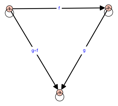
# A Simple Category: with composition and identity morphisms
G = DiGraph( {1 : [1], 2 : [2], 3 : [3]})
G.add_edges([(1, 2, "f"), (2, 3, "g"), (1, 3, "g∘f")  ])
G.show(edge_labels=True) 

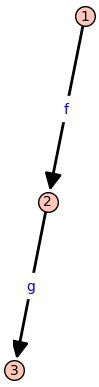
# This graph is not a category because there is no explicit composition 
G = DiGraph()
G.add_edges([(1, 2, "f"), (2, 3, "g")])  # Missing (1, 3, "g∘f")
G.show(edge_labels=True)

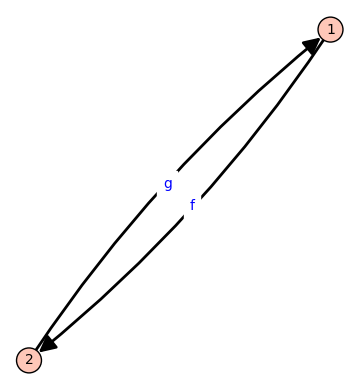
# This graph is not a category because it lacks identity morphisms
G = DiGraph()
G.add_edges([(1, 2, "f"), (2, 1, "g")])  # No identity morphisms
G.show(edge_labels=True)

Categories .VS. DAGs(Graph Theory)

Property	DAG	Category
Directed edges	✅	✅
No cycles	✅	❌ Not always
Self-loops allowed?	❌ No	✅ Yes (identity morphisms)
Must have composable paths?	❌ No	✅ Yes

If a category has no isomorphisms (self-loops) and only strictly hierarchical structure, it could be a DAG.

• e.g. A preorder category, where there is at most one morphism between any two objects and no reversibility, can be represented as a DAG.

• A poset category is always a DAG because it models partial ordering.

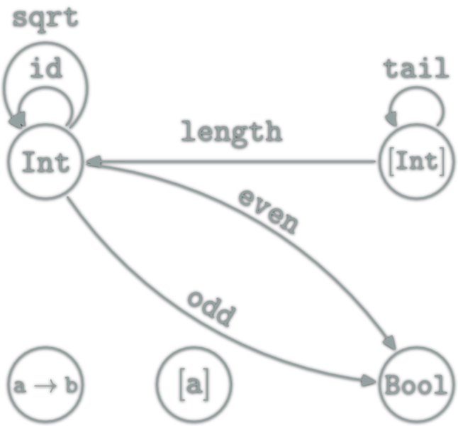
Functor: structure preserving mapping between categories (like rebuilding an organisation)

• In Haskell, functor can be seen as boxes containing all types and functions. Haskell types look like a fractal(can replicate).

Category Theory oriented Programming:

• Focus on the type and operators

• Extreme generalisation and better modularity

9.1.3. FP Wolfram Language: from Functional Programming

(*OOP*)
data={a,b,c};
Do[
   data[[k]]=f[data[[k]]], {k,Length[data]}
];
data
(*FP*)
Map[f,{a,b,c}]
f /@ {a,b,c}

Map[f, {{1,2,3},{4,5,6},{7,8,9}}] 
Map[f, {{1,2,3},{4,5,6},{7,8,9}}, {1}] 
Map[f, {{1,2,3},{4,5,6},{7,8,9}}, {2}] (*{2} indicates level 2*)

Map[Reverse, {{1,2,3},{4,5,6},{7,8,9}}] (*With-In*)
Map[Reverse, {{1,2,3},{4,5,6},{7,8,9}}, {1}] 
Reverse[{{1,2,3},{4,5,6},{7,8,9}}] (*Between*)

Map[Sort, {{2,1,3},{a,c,b},{7,2,8}}]
Sort[{{2,1,3},{a,c,b},{7,2,8}}]

Apply[g,f[1,2,3]]
g @@ f[1,2,3]
Apply[g, {{1,2,3},{4,5,6},{7,8,9}}, {1}]

Apply[Rule,{x,5}] (*a -> 1 is read as "a maps to 1"*)
Apply[Rule, {{a,1},{b,2},{c,3}}, {1}] (*turn pairs into a list of rules*)
Rule @@@ {{a,1},{b,2},{c,3}}

Nest[f,x,3]
NestList[f,x,3]
Nest[(1+r)# &, A, 5]
NestList[(1+r)# &, A, 5]

NestList[1.1#&, 100, 5]

FixedPoint[(#+2/#)/2 &, 1.0]
FixedPointList[(#+2/#)/2 &, 1.0]

ListPlot[FixedPointList[(# + 2/#)/2 &, 1.0], 
        PlotStyle -> {Blue, PointSize[Medium]}, 
        GridLines -> Automatic, 
        AxesLabel -> {"Iteration", "Value"}, 
        PlotRange -> All]

Fold[f,x,{a,b,c}]
FoldList[f,x,{a,b,c}]
FoldList[Max,{1,5,2,4,7,9,1,1}]

Map[(#+x)&,{1,2,3,4,5}]
{1,2,3,4,5}+x
Apply[Plus,{1,2,3,4,5}]
Total[{1,2,3,4,5}]

FoldList[Plus,{1,2,3,4,5}]
Accumulate[{1,2,3,4,5}]
Total[{{1,1,1},{2,2,2},{3,3,3}}]

Map[Select[#,EvenQ]& , {{1,2,3},{4,5,6},{7,8,9}}]
Map[Select[  EvenQ]  , {{1,2,3},{4,5,6},{7,8,9}}]

f[p_]:=Select[p,EvenQ]
Map[f , {{1,2,3},{4,5,6},{7,8,9}}]

f = If[#==0 , 1 , # f[#-1]] &; (* #和f 中间空格表示乘号 *)
f[5] (* 5!=120 *)

120

Clear[f]
MapThread[f,{{a,b,c},{x,y,z}}]
BlockMap[f,{1,2,3,4,5,6,7,8,9}, 3]

BlockMap[f,{1,2,3,4,5,6,7,8,9}, 3,1]
ArrayFilter[f,{1,2,3,4,5,6,7,8,9}, 1, Padding->None]
ArrayFilter[Mean,{1,2,3,4,5,6,7,8,9}, 1, Padding->None] 

9.2. Coding Theory & Information

symbols<->info, data storage/compression/transmission/cryptography, error detection/correction to protect information

9.3. Data analysis

Visualisation, Simulation

9.4. Statistics & Probability Theory(SPT)

Descriptive, Inferential, Correlation & Regression, Sample Spaces (countable VS. uncountable), Conditional Probability, Random Variable

Math built SPT through two ways:

• Discrete approach through combinatorics

• Continuous approach through measure theory (e.g. modelling Stochastic Processes正态分布，是一种模型，对binomial分布进行模拟)

9.5. Game Theory & Decision & Operation

Utilities/Strategies, Decision Analysis, Optimization, Stochastic Process Modeling

9.6. Quantum Theory

This is cornerstone of modern physics, with deep roots in Linear Algebra, Functional Analysis, DE, Complex Analysis, Group Theory, Probability & Statistics, Topology, Measure and Variational Calculus